Strategies to Reduce False Positives in Virtual Screening: A Guide for Drug Discovery Scientists

Abstract

This article provides a comprehensive guide for researchers and drug development professionals on addressing the pervasive challenge of false positives in structure-based virtual screening. It explores the fundamental causes and impacts of false positives, reviews cutting-edge methodological advances including machine learning classifiers and consensus scoring models, and offers practical troubleshooting and optimization protocols. The content is validated through comparative analysis of state-of-the-art tools and prospective case studies, delivering actionable strategies to significantly improve hit rates and screening efficiency in early drug discovery.

Understanding the False Positive Problem: Why Most Virtual Screening Hits Fail

Frequently Asked Questions

What is a false positive in the context of virtual screening? In virtual screening, a false positive is a compound that is computationally predicted to be active against a biological target but fails to show activity in subsequent experimental validation [1] [2]. These compounds consume significant time and resources, as they must be synthesized or acquired and then tested experimentally, only to be invalidated.

Why are false positives such a persistent problem? False positives persist due to fundamental limitations in computational models. Scoring functions, which predict binding affinity, can be inaccurate and sometimes fail to account for critical factors such as the role of water molecules in the binding site, ligand strain energy, and unfavorable desolvation penalties [2]. Even advanced rescoring techniques, including those using quantum mechanics, have not yet solved this problem globally [2].

Can machine learning completely eliminate false positives? While machine learning shows significant promise, it has not eliminated the false positive problem. Its performance is highly dependent on the quality and rigor of the training data. If the model is trained on decoy compounds that are too easy to distinguish from actives, it will not perform well in real-world prospective screens where distinguishing truly compelling decoys is the challenge [3]. When trained effectively, machine learning can substantially improve hit rates [3].

What is the most effective strategy to manage false positives? A powerful and robust strategy is the combination of virtual screening with a highly accurate experimental validation technique, such as Surface Plasmon Resonance (SPR). Virtual screening rapidly narrows a library of millions of compounds down to a few hundred or dozen promising candidates. SPR then acts as a "rigorous practical exam," providing label-free, quantitative data on which compounds truly bind to the target protein, effectively filtering out false positives before more costly cellular or functional assays are conducted [1].

Troubleshooting Guides

Guide 1: Diagnosing and Addressing High False Positive Rates in Your Virtual Screening Workflow

A high false positive rate indicates a disconnect between your computational predictions and biological reality. Use this guide to identify and correct common pitfalls.

Problem Area	Symptoms	Diagnostic Checks	Corrective Actions
Scoring Function Limitations	- High enrichment in docking scores but no activity in assays.- Poor correlation between score and binding affinity in validation.	- Benchmark multiple scoring functions on known actives/inactives for your target.- Check if your hit compounds have strained conformations or unsatisfied polar groups.	- Use consensus scoring from multiple functions [2].- Apply post-docking filters for undesirable chemical features [2].
Inadequate Pose Prediction	- Putative hits have unrealistic binding geometries.- Lack of key interactions seen in crystal structures of known actives.	- Perform visual inspection of top-ranked poses against a known reference structure.- Check for clashes and incorrect binding modes.	- Use a docking method with high pose prediction accuracy (e.g., >90% [4]).- Incorporate water molecules in the binding site if critical for binding [4].
Training Data for ML Models	- Your ML classifier performs well retrospectively but fails prospectively.	- Audit your training set: are the decoys too easy to distinguish from actives? [3]	- Retrain your model using a dataset of "compelling decoys" that closely mimic true binders [3].

Guide 2: Implementing a Tiered Experimental Validation Protocol to Filter False Positives

This protocol outlines a step-wise experimental strategy to efficiently triage computational hits and focus resources on the most promising leads.

Validation Stage	Primary Objective	Key Technique(s)	Key Outcome & Decision Point
Primary Biophysical Validation	Confirm direct, specific binding to the target protein.	Surface Plasmon Resonance (SPR) [1]	Output: Quantitative binding affinity (KD), kinetics (Kon, Koff).Decision: Proceed with compounds that show direct, measurable binding.
Secondary Functional Validation	Assess biological activity in a target-specific assay.	Biochemical Activity Assay (e.g., enzyme inhibition) [3]	Output: Half-maximal inhibitory concentration (IC50).Decision: Prioritize compounds with potent activity for further testing.
Tertiary Cellular & Phenotypic Validation	Evaluate effect in a cellular context and check for cytotoxicity.	Cell-Based Assay (e.g., reporter gene, phenotypic readout) [1]	Output: Efficacy in cells and therapeutic index.Decision: Advance compounds with desired cellular activity and low toxicity.

Experimental Data & Protocols

Quantitative Performance of Screening Methods

The following table summarizes the effectiveness of different approaches as reported in recent studies, providing benchmarks for your own work.

Method / Strategy	Key Metric	Performance Outcome	Context & Notes
Traditional VS + Expert Picking [3]	Hit Rate (Active Compounds)	~12%	Median performance across 54 successful campaigns; highlights the "baseline" for the field.
vScreenML Classifier (Prospective) [3]	Hit Rate (Active Compounds)	~43% (10 of 23 compounds with IC50 < 50 μM)	Machine learning model trained on "compelling decoys"; demonstrates a significant improvement.
VS + SPR Workflow [1]	Experimental Validation Rate	32.5% (13 of 40 VS hits confirmed by SPR)	A concrete example where SPR filtered out over 65% of virtual screening hits, drastically focusing efforts.
Glide WS (Docking Method) [4]	Self-Docking Accuracy	92% (vs. 85% for Glide SP)	Improved pose prediction can lead to better virtual screening enrichment and reduced false positives.

Detailed Protocol: Integrated Virtual Screening and SPR Validation

This protocol is adapted from a successful case study that identified a potent PPARγ inhibitor [1].

Objective: To rapidly and reliably identify true small-molecule binders for a protein target from a large compound library.

Workflow Overview:

Step-by-Step Methodology:

• Virtual Screening Pre-screening:

  • Target Preparation: Obtain a high-resolution crystal structure of your target protein (e.g., from the PDB). Clean the structure, add hydrogen atoms, and define the binding site residue.
  • Library Preparation: Prepare a database of compounds in a suitable format for docking. This could be a commercially available library (e.g., ~23,000 compounds [1]) or an ultra-large virtual library.
  • Multi-Stage Docking: Perform a structured virtual screening to balance computational cost and accuracy.
    • Stage 1 (HTVS): Dock the entire library using a fast, high-throughput method. Select the top 10% of compounds.
    • Stage 2 (SP): Redock the selected compounds using a standard precision method. Select the top 10% from this stage.
    • Stage 3 (XP): Redock the final subset using an extra precision method. From this, select the top-ranked compounds (e.g., 40 compounds) for experimental testing [1].

• SPR Experimental Validation:

  • Sample Preparation: Purify the target protein to homogeneity. Prepare DMSO stocks of the shortlisted compounds.
  • Single-Concentration Screening: Immobilize the target protein on an SPR sensor chip. Test each compound from the virtual screening shortlist at a single concentration to obtain a binding response. Compare the response to a known positive control [1].
  • Kinetic Analysis: For compounds that show binding above the control threshold, perform a concentration-series experiment. This involves injecting a range of concentrations of the compound to obtain binding curves. Fit this data to a model to determine the equilibrium dissociation constant (KD), and the association (Kon) and dissociation (Koff) rates [1].

• Downstream Functional Assays:

  • Activity Validation: Test the SPR-confirmed binders in a biochemical assay relevant to the target's function (e.g., an enzyme inhibition assay) to determine IC50 values [3].
  • Cellular Validation: Finally, validate the most potent compounds in a cell-based model to confirm the biological activity translates to a more complex, physiological environment [1].

The Scientist's Toolkit: Research Reagent Solutions

Essential Material / Tool	Function in the Context of False Positive Reduction
Structure-Based Docking Software (e.g., Glide, Schrödinger) [1] [4]	Predicts the binding mode and affinity of small molecules to a protein target, enabling the rapid screening of ultra-large virtual libraries.
Structured Compound Libraries (e.g., MCE Bioactive Library) [1]	Provides a curated, diverse, and often drug-like set of compounds for screening, improving the odds of finding genuine hits.
Surface Plasmon Resonance (SPR) Instrument [1]	A gold-standard biophysical technique that provides label-free, quantitative data on binding affinity and kinetics, serving as a critical filter for false positives.
Machine Learning Classifiers (e.g., vScreenML) [3]	Trained on challenging datasets, these tools can distinguish true binders from "compelling decoys" with higher accuracy than traditional scoring functions.
Crystallographic Structures (PDB) [3]	Provides the experimental 3D structure of the protein target, which is essential for structure-based screening and for understanding true binding interactions.

Quantitative Data on Virtual Screening Performance

Understanding the typical hit rates and the factors that influence them is crucial for setting realistic expectations and quantifying the problem of false positives in virtual screening (VS). The table below summarizes key quantitative findings from large-scale VS studies.

Table 1: Virtual Screening Hit Rates and Impact of Library Scale

Metric	99 Million-Molecule Library	1.7 Billion-Molecule Library	Implication
Molecules Tested	44 molecules [5]	1,521 molecules [6] [5]	Larger scales enable more reliable statistics.
Observed Hit Rate	11.4% (5 hits from 44 tested) [5]	22.4% (290 hits from 1,294 tested) [5]	Hit rate can improve substantially with larger libraries.
Potency of Hits	Activities from 1.3 to 400 µM [5]	168 inhibitors with Ki < 166 µM [6]	Larger libraries can yield more potent inhibitors.
Recommended Minimum Tested	Not specified	>100 molecules [5]	Testing several hundred molecules is needed for hit rates to converge and for reliable results [6].

The economic impact of false positives extends beyond virtual screening. The table below outlines costs associated with false positives in a different, but related, context: clinical cancer screening. These figures illustrate the broader economic burden of false-positive results in life sciences.

Table 2: Economic Impact of False-Positive Cancer Screens

Cost Category	Findings from the Prostate, Lung, Colorectal, and Ovarian (PLCO) Cancer Screening Trial
Frequency of False Positives	43% of the study sample incurred at least one false-positive screen [7].
Follow-up Care Rate	83% of patients with a false-positive screen received follow-up care [7].
Additional Medical Costs	Adjusted mean difference in medical care expenditures in the year following a false-positive screen was $1,024 for women and $1,171 for men [7].
Non-Medical Costs (Time)	For a false-positive lung cancer screen, patients spent a mean of 1.5 hours receiving care [7].

Troubleshooting Guides and FAQs

Frequently Asked Questions

Q1: Our virtual screening campaign produced a high number of false positives. What are the primary reasons for this? False positives in VS arise from several well-documented challenges in scoring and pose prediction [8]. Common reasons include:

• Inaccurate Scoring Functions: Scoring functions are widely known to be inaccurate and often struggle to correctly calculate binding affinities, failing to distinguish true binders from decoys [2].
• Incorrect Ligand Poses: The docking process may generate poses that are not physiologically relevant, featuring strained conformations or unsatisfied hydrogen bonds [2].
• High Ligand Strain Energy: The predicted binding pose might require the ligand to adopt a high-energy conformation, which is unfavorable for actual binding.
• Inadequate Treatment of Solvation: The models may not properly account for the favorable or unfavorable contributions of water molecules being displaced upon ligand binding [2].
• Presence of Artifacts: Top-ranking molecules can sometimes be compounds that act as aggregation-based inhibitors or interfere with the assay, rather than true binders [9].

Q2: We have limited resources and can only test a small number of compounds. How many should we test to have confidence in our results? Based on large-scale validation studies, it is recommended to test at least 100 molecules from a virtual screen to achieve reliable results and identify high-affinity hits [5]. Testing only a few dozen compounds leads to high variability and unreliable hit rate estimates. Simulations show that confidence in the true hit rate increases significantly when several hundred molecules are tested [6] [5].

Q3: Does using a larger virtual library automatically lead to better results? While larger libraries (billions of molecules) have been shown to improve hit rates, discover more scaffolds, and yield more potent inhibitors [6] [5], they also amplify the challenge of false positives. As libraries grow, the absolute number of false positives also increases, and they can come to dominate the top-scoring lists if not properly managed [9]. Therefore, larger libraries are beneficial but must be paired with careful analysis and filtering.

Q4: We've tried multiple scoring functions and found they don't agree. What is the value of consensus scoring? While consensus scoring is a popular strategy, evidence suggests it may not be a silver bullet. A systematic study found that neither semi-empirical quantum mechanics potentials, force fields with implicit solvation, nor empirical machine-learning scoring functions could reliably discriminate true positives from false positives [2]. Refining poses with molecular mechanics also provided only marginal improvement. This underscores that the problem is complex and no single rescoring method has yet proven globally effective.

Troubleshooting Guide: Mitigating False Positives

Problem: An unmanageably large number of top-ranking hits from docking, many of which are likely false positives. Solution: Implement a hierarchical workflow that filters results based on multiple criteria beyond the docking score.

• Step 1: Apply Property and Pan-Assay Interference Compound (PAINS) Filters. Remove compounds with undesirable chemical properties or functional groups known to cause assay interference.
• Step 2: Visually Inspect Top-Ranked Poses. An experienced computational chemist should visually examine the predicted protein-ligand complexes. Look for:
  • Physiologically reasonable ligand conformations.
  • Satisfaction of key hydrogen bonds.
  • Appropriate placement of hydrophobic groups in apolar pockets.
  • Absence of severe steric clashes [2].
• Step 3: Prioritize Diverse Chemotypes. Instead of selecting the top 100 hits, choose the top 20-30 from several distinct chemical scaffolds to diversify your chances of success and avoid testing multiple analogs of the same false positive.
• Step 4: Use Expert Knowledge. Incorporate any existing structure-activity relationship (SAR) data or knowledge about the target's binding site to select compounds that have features known to be important for activity [8].

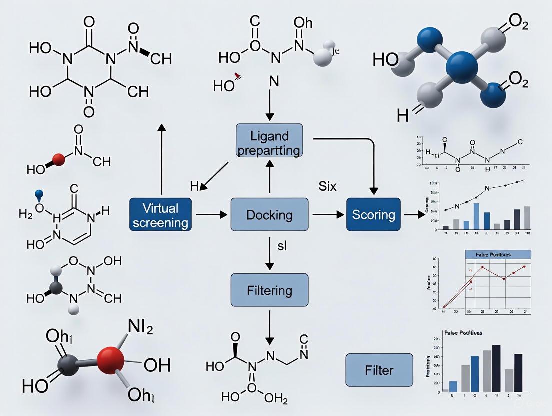
Workflow Visualization

The following diagram illustrates a recommended virtual screening workflow designed to mitigate false positives, from initial preparation to experimental testing.

The Scientist's Toolkit: Key Research Reagents & Materials

Table 3: Essential Reagents and Software for Virtual Screening

Item / Resource	Function / Description	Example Tools / Vendors
Virtual Compound Libraries	Large collections of purchasable and readily synthesizable compounds for screening.	ZINC [8], Enamine "make-on-demand" [5]
Protein Structure Files	Experimentally determined 3D structures of the target protein.	Protein Data Bank (PDB) [8]
Structure Validation Software	Tools to check the reliability of crystallographic models, especially in the binding site.	VHELIBS [8]
Conformer Generator	Software to predict the low-energy 3D conformations of molecules for docking.	OMEGA, ConfGen, RDKit (ETKDG) [8]
Molecule Standardizer	Tools to prepare 2D structures, defining correct protonation states, charges, and removing salts.	Standardizer, LigPrep, MolVS [8]
Docking & Scoring Software	The core computational engine for predicting how ligands bind to the protein and ranking them.	DOCK [6] [5]
Visualization Software	Essential for expert inspection of docking poses and rational decision-making.	Flare, Maestro, VIDA [8]

Troubleshooting Guides

Why does my virtual screening yield a high rate of false positives?

A high false-positive rate is often the result of fundamental limitations in traditional scoring functions and the generation of unrealistic ligand poses [3].

• Problem: Traditional scoring functions struggle to accurately predict binding affinities. They can be overly simplistic, may be overtrained on limited datasets, or fail to consider critical non-linear interactions between energy terms [3].
• Symptoms: Many top-scoring compounds from a virtual screen show no activity in subsequent biochemical assays. The literature indicates a median hit rate of only about 12% when these functions are used [3].
• Diagnosis: The primary issue is that standard scoring functions are not trained to distinguish truly "active" complexes from "compelling decoys"—inactive compounds that nonetheless appear to be good binders in docking poses. If a model is trained on decoys that are easily distinguishable from actives (e.g., due to steric clashes or poor packing), it will perform poorly in real-world applications where decoys are more sophisticated [3].

Resolution

• Implement Advanced Classifiers: Move beyond regression models that predict affinity. Use a machine learning classifier, like vScreenML, specifically trained to discriminate between active complexes and challenging decoy complexes. In a prospective screen against acetylcholinesterase, this approach led to a hit where nearly all candidate inhibitors showed detectable activity, with one compound reaching an IC50 of 280 nM [3].
• Use a Rigorous Training Set: Employ a dedicated training strategy such as the D-COID dataset. This strategy involves matching available active complexes from the PDB with highly compelling, individually matched decoy complexes that mimic the types of poses encountered in real virtual screens [3].
• Validate Prospectively: Always validate a new scoring method or classifier in a prospective experimental screen within the same study to avoid the common pitfall of overfitting and ensure the model's performance is transferable [3].

How can I generate more convincing decoy complexes for machine learning?

The quality of your decoy set is paramount for training an effective classifier [3].

• Problem: If decoy complexes are not "compelling," a machine learning model will learn to exploit trivial differences (e.g., the presence of steric clashes or systematic under-packing in decoys) rather than the nuanced physics of binding. This leads to a model that performs well on benchmarks but fails in real-world applications [3].
• Symptoms: Your classifier achieves high accuracy during retrospective benchmarking but fails to identify active compounds in a prospective screen.

Resolution

• Source Actives from Reliable Structures: Compile your set of active complexes from high-quality crystal structures in the Protein Data Bank (PDB). This ensures the model learns from correct protein-ligand interactions. Filter these ligands to adhere to the same physicochemical properties required for your actual screening library [3].
• Create Matched Decoys: For each active complex, generate decoys that are individually matched and highly compelling. The decoys should be structurally similar to actives but lack the specific interactions required for true binding. The D-COID dataset construction strategy is designed for this purpose [3].
• Minimize Complexes: Subject both active and decoy complexes to energy minimization before training. This prevents the model from simply distinguishing between crystal structures and docked models, forcing it to learn more generalizable features of binding [3].

Frequently Asked Questions (FAQs)

What is the typical hit rate I should expect from a structure-based virtual screen?

A review of 54 successful virtual screening campaigns revealed a median hit rate of approximately 12%. This means that, on average, only about 12% of the top-scoring compounds selected for experimental testing show confirmable activity in biochemical assays. The most potent initial hit from these campaigns typically had a Kd or Ki value of around 3 µM [3].

What is the key difference between a regression model and a classifier for virtual screening?

• Regression Models: These are trained to recapitulate the known binding affinities (e.g., Kd, Ki) of protein-ligand complexes. A significant limitation is that they are never explicitly trained on inactive (decoys) complexes during the training process [3].
• Binary Classifiers: These are trained to distinguish between two categories: "active" complexes and "inactive" or "decoy" complexes. This approach is often more appropriate for virtual screening, where the primary task is to sift through a large library of mostly inactive compounds to find the few true actives [3].

What are common reasons for the disappointing performance of machine learning scoring functions?

Two major artifacts can inflate benchmark performance and lead to poor real-world results [3]:

• Information Leakage: This occurs when the validation or testing data are not truly independent of the training data, leading to overfitting. The model memorizes the training data rather than learning generalizable rules.
• Detecting Chemical Bias: Some models may inadvertently learn systematic differences in the chemical properties of the active versus decoy compound sets, rather than learning the structural determinants of binding from the protein-ligand complex structures.

Experimental Data & Protocols

Performance Comparison: Traditional vs. Machine Learning Approaches

The table below summarizes key performance metrics from a prospective virtual screening study using the vScreenML classifier against the acetylcholinesterase (AChE) target [3].

Metric	Traditional Scoring (Typical Median)	vScreenML (Prospective AChE Screen)
Hit Rate	~12% of tested compounds show activity [3]	Nearly all candidates showed detectable activity [3]
Number of Active Compounds	Not Specified	23 compounds tested [3]
Potency of Most Active Hit	~3 µM (Kd/Ki) [3]	280 nM (IC50), Ki = 173 nM [3]
Number of Potent Hits	Not Specified	10 compounds with IC50 < 50 µM [3]

Experimental Protocol: Prospective Validation on AChE

This protocol details the key experimental steps from the vScreenML prospective validation study [3].

1. Virtual Screening with vScreenML

• Objective: Identify candidate inhibitors of acetylcholinesterase (AChE) from a chemical library.
• Method: The compound library was docked against the 3D structure of AChE. The resulting protein-ligand complexes were then scored using the pre-trained vScreenML classifier. The top-ranking compounds based on the classifier's score were selected for experimental testing.

2. Experimental Validation via Biochemical Assay

• Objective: Experimentally measure the inhibitory activity of the top-scoring virtual hits.
• Methodology:
  • Assay Type: Biochemical inhibition assay.
  • Target: Acetylcholinesterase (AChE).
  • Measurement: Determine the half-maximal inhibitory concentration (IC50) for each compound.
  • Calculation: For the most potent inhibitor, the inhibition constant (Ki) was calculated from the IC50 value.

Workflow and Pathway Diagrams

Virtual Screening Workflow: Traditional vs ML Approach

D-COID Training Strategy for Robust ML Models

The Scientist's Toolkit: Research Reagent Solutions

Item	Function in Virtual Screening Research
D-COID Dataset	A specialized training dataset designed to build effective machine learning classifiers. It provides a set of active protein-ligand complexes paired with highly compelling, individually matched decoy complexes to teach models to distinguish true binders from sophisticated non-binders [3].
vScreenML Classifier	A general-purpose machine learning classifier for virtual screening, built on the XGBoost framework. It is trained using the D-COID strategy to evaluate docked protein-ligand complexes and score them based on their likelihood of being active [3].
Protein Data Bank (PDB)	A critical source for high-quality, experimentally determined 3D structures of protein-ligand complexes. These structures are used as reliable examples of "active" complexes for training and benchmarking scoring functions and classifiers [3].
Acetylcholinesterase (AChE) Biochemical Assay	A standard experimental method used for the prospective validation of virtual screening hits. It measures the half-maximal inhibitory concentration (IC50) of candidate compounds to confirm and quantify their biological activity against the AChE target [3].

FAQs: Understanding Data Quality in Virtual Screening

What is the "Decoy Dilemma" in virtual screening? The "Decoy Dilemma" refers to the significant challenge where the use of poorly designed or biased decoy molecules (presumed inactive compounds) in training machine learning models for virtual screening leads to high false positive rates and an over-optimistic estimation of a model's predictive performance. This occurs because models learn to recognize superficial patterns in the decoys rather than true binding interactions, compromising their ability to identify real hits in experimental validation [10].

How do false positives impact the drug discovery process? False positives in virtual screening have substantial practical consequences. They consume significant wet-lab time and reagents, as most compounds selected in ultra-large virtual screening campaigns turn out to be inactive when characterized in biochemical assays. While false negatives represent missed opportunities, false positives incur very real expenses. For example, hit rates for non-GPCR targets are typically low, with one screen of 235 million compounds against SARS-CoV-2 main protease yielding only 3 hits from 100 compounds tested (3% hit rate) [11].

What are the main causes of data quality issues in training datasets? Data quality issues stem from several sources: inconsistent data collection leading to biases, hidden biases in commonly used decoy sets like DUD-E, mislabeled compounds, and datasets that fail to adequately represent the vast chemical space of real-world compounds. These imperfections mean models learn from noisy or erroneous patterns rather than true structure-activity relationships [12] [10].

Can more sophisticated AI algorithms compensate for poor-quality data? No. Evidence shows that superior performance comes from better data quality and representation rather than more complex algorithms. One study achieved 99% accuracy with a conventional support vector machine (SVM) algorithm using optimized data, far surpassing performances of virtual screening platforms using sophisticated deep learning methods. This highlights that poor understanding and erroneous use of chemical data—not deficiencies in AI algorithms—typically leads to poor predictive performance [10].

Troubleshooting Guides

Problem: High False Positive Rates in Virtual Screening

Symptoms

• Computationally selected compounds fail to show activity in experimental assays
• High initial hit rates in silico that don't translate to wet-lab validation
• Models perform well on benchmark tests but poorly in real-world applications

Diagnostic Steps

Step	Action	Expected Outcome
1	Audit decoy set composition	Identify hidden biases or inappropriate properties in decoys
2	Analyze chemical space coverage	Verify adequate representation of relevant chemical space
3	Check for label consistency	Identify mislabeled active/inactive compounds
4	Test model on external validation sets	Assess generalizability beyond training data

Solutions

• Implement Data-Centric Validation: Systematically assess the properties of chemical data, including representation, quality, quantity, and composition [10].
• Use Multiple Receptor Conformations: Account for receptor flexibility by docking to multiple distinct receptor structures, then select only intersection ligands that rank highly across all conformations [13].
• Apply Advanced Machine Learning Classifiers: Use tools like vScreenML 2.0, which is specifically trained to distinguish active complexes from carefully curated decoys that would otherwise represent false positives [11].
• Improve Data Representation: Employ merged molecular representations (e.g., Extended+ECFP6 fingerprints) rather than single representations for better molecular description [10].

Problem: Model Performance Doesn't Generalize to New Targets

Symptoms

• Excellent performance on training and validation data
• Poor performance when applied to novel target classes
• Inability to identify true binders for structurally diverse proteins

Solutions

• Expand Training Diversity: Incorporate newly released structures from protein data banks and include additional features for enhanced discriminative power [11].
• Implement Robust Feature Selection: Identify and use the most important structural and interaction features rather than all possible features to prevent overfitting and improve generalization [11].
• Utilize Physics-Based Methods: Combine machine learning with physics-based docking approaches like RosettaVS that model receptor flexibility and incorporate both enthalpy and entropy calculations [14].

Experimental Protocols & Methodologies

Protocol 1: Multiple Receptor Conformation (MRC) Screening for False Positive Reduction

Purpose: To reduce false positives in structure-based virtual screening by accounting for receptor plasticity through the use of multiple distinctive receptor structures.

Materials

• Receptor structures (crystal structures or MD simulation outputs)
• Chemical compound library for screening
• Docking software (e.g., GOLD)
• Control molecules (high-affinity and low-affinity controls)

Procedure

• Generate Multiple Receptor Conformations: Explore structural flexibility using molecular dynamics simulations. Extract distinctive structures from trajectory data [13].
• Prepare Receptor Models: Use resultant distinctive structures and crystal structure as receptor models for docking exercises [13].
• Dock Compound Library: Separately dock the entire molecule library (including control molecules) to each conformation of the receptor using appropriate docking software [13].
• Rank and Select Intersection Ligands: For each receptor model, generate a top-ranked molecule list. Select only the common members that appear in all top-ranked lists from all receptor models [13].
• Experimental Validation: Test selected intersection molecules for binding affinity to verify true positive identification.

Expected Results: This selection strategy successfully distinguishes high-affinity and low-affinity control molecules and identifies true binders while excluding false positives that only rank highly in some receptor conformations [13].

Workflow: MRC Screening for False Positive Reduction

Protocol 2: Machine Learning Classification with vScreenML 2.0

Purpose: To implement an improved machine learning classifier that reduces false positives in structure-based virtual screening by distinguishing active complexes from decoys.

Materials

• Protein-ligand complex structures
• vScreenML 2.0 software (Python implementation)
• Curated training dataset with active compounds and decoys
• Feature calculation tools

Procedure

• Feature Calculation: Compute key molecular features including ligand potential energy, buried unsatisfied atoms for select polar groups in ligand, additional 2D structural features of ligands, complete characterization of interface interactions in protein-ligand complexes, and pocket-shape features [11].
• Feature Selection: Identify and use the 49 most important features to ensure model generalization and avoid overtraining, rather than using all 165 available features [11].
• Model Training: Train the classifier on carefully curated datasets of active complexes and decoys, incorporating newly released structures from PDB [11].
• Model Application: Apply the trained model to score protein-ligand complexes from virtual screening, with active complexes receiving scores close to 1 and decoy complexes receiving scores close to 0 [11].
• Hit Selection: Prioritize compounds with high scores for experimental validation.

Expected Results: vScreenML 2.0 demonstrates dramatically improved performance over traditional methods, with higher recall (0.89 vs. 0.67 in original) and Matthews correlation coefficient (0.89 vs. 0.69 in original), significantly reducing false positive rates [11].

Workflow: vScreenML 2.0 Classification Process

Data Presentation

Virtual Screening Performance Comparison Across Methods

Table 1: Performance metrics of various virtual screening approaches for reducing false positives

Method	Key Principle	Performance Metrics	Advantages	Limitations
Multiple Receptor Conformations [13]	Selects intersection ligands ranking highly across all receptor conformations	Successfully identified 14/14 high-affinity controls for T-loop pocket; 7/7 for RNA binding site	Accounts for receptor plasticity; Reduces conformation-specific false positives	Computationally intensive; Requires multiple quality structures
vScreenML 2.0 [11]	Machine learning classifier trained to distinguish actives from decoys	MCC: 0.89; Recall: 0.89; Significant improvement over original vScreenML (MCC: 0.69)	Dramatically reduces false positives; Improved generalizability	Requires careful feature selection and curation
RosettaVS with Active Learning [14]	Physics-based docking with active learning for ultra-large libraries	EF1%: 16.72 (vs. 11.9 for second-best method); High accuracy in pose prediction	Models full receptor flexibility; Efficient for billion-compound libraries	Complex implementation; Computational resource demands
Data-Centric AI with Conventional ML [10]	Focus on data quality over algorithm complexity	99% accuracy with SVM vs. complex deep learning methods	Emphasizes interpretability; Challenges assumption that complex AI is always better	Requires significant data curation expertise

Research Reagent Solutions for False Positive Reduction

Table 2: Essential tools and resources for implementing effective false positive reduction strategies

Resource	Type	Function in False Positive Reduction	Access
GOLD Software [13]	Docking software	Used for molecular docking exercises with multiple receptor conformations	Commercial
RosettaVS [14]	Virtual screening platform	Implements high-speed docking modes (VSX, VSH) and active learning for ultra-large libraries	Open-source
vScreenML 2.0 [11]	Machine learning classifier	Distinguishes active complexes from decoys using optimized feature set	Open-source
DUD-E Dataset [10]	Benchmark decoy set	Provides decoy molecules for training and testing (with caution for hidden biases)	Public
Otava PrimScreen1 Library [13]	Diversity molecule library	Used for validation of screening approaches with known controls	Commercial
BALL Framework [15]	Computational library	Provides tools for ligand/receptor preparation, scoring, docking, and QSAR analysis	Open-source

In the field of drug discovery, virtual screening (VS) serves as a critical computational technique to identify potential hit compounds from extensive molecular libraries by predicting their binding affinity to a biological target [8] [16]. While this approach significantly reduces the time and resources needed for initial screening phases compared to traditional high-throughput methods, it faces a substantial challenge: high false positive rates [13]. False positives occur when compounds are incorrectly predicted to be active, leading researchers down unproductive experimental pathways. The repercussions include wasted synthetic efforts, misallocated assay resources, and delayed project timelines, presenting a major bottleneck in early drug discovery [17] [13]. This case study examines the root causes of false positives in virtual screening campaigns and presents proven strategies to mitigate them, enabling more efficient and cost-effective drug discovery.

False positives in virtual screening can originate from various methodological and technical limitations. Understanding these sources is the first step toward developing effective countermeasures.

• Receptor Rigidity and Plasticity: Traditional structure-based virtual screening (SBVS) often treats the protein receptor as a rigid structure. However, this simplification can lead to inaccurate ligand binding energy estimations and poor binding mode predictions, as it fails to account for the natural flexibility and dynamics of the protein [13]. Conversely, while using multiple receptor conformations (MRCs) addresses this issue, each distinct conformation introduced can bring its own set of false positives, complicating the selection of true ligands [13].

• Compound Interference in Indirect Assays: Many biochemical assays used for experimental validation rely on indirect detection methods, particularly coupled enzyme systems. In these systems, a test compound might inhibit or interfere with the coupling enzymes rather than the target enzyme itself, generating a false signal of activity [17]. For example, in common kinase assays that use luciferase-based detection, compounds that inhibit luciferase can appear as false positives for kinase inhibition.

• Inadequate Compound Preparation and Conformational Sampling: The preparation of compound libraries for virtual screening requires careful attention to molecular details. If the bioactive conformation of a compound is not included among the generated conformers, it may be incorrectly dismissed. Conversely, generating high-energy conformations that have a low probability of being accessed at room temperature can be misleading and cause false positive results [8]. Proper definition of protonation states, tautomers, and stereochemistry is equally crucial.

• Limitations of Specific VS Methodologies: Certain virtual screening approaches are inherently more prone to false positives. Pharmacophore modeling, for instance, has been noted to often suffer from a high false positive rate, meaning a low proportion of virtual hits hold up under experimental verification [16]. Similarly, oversimplified similarity methods may extrapolate poorly beyond a very short distance in chemical space [16].

Quantitative Impact: The Real Cost of False Positives

The impact of false positives is not merely theoretical; it has direct, measurable consequences on screening efficiency and resource allocation. The following table summarizes the potential resource impact of false positives in a typical high-throughput screening (HTS) campaign.

Table 1: Resource Impact of False Positives in a Hypothetical HTS Campaign of 250,000 Compounds

Metric	Coupled Enzyme Assay (1.5% FPR)	Direct Detection Assay (0.1% FPR)	Impact Reduction
False Positive Leads	3,750	250	15-fold (93%)
Re-screening Costs	High	Low	Significant savings
Project Timeline	Delayed (weeks)	Accelerated	Improved efficiency
SAR Confusion	High	Low	More reliable optimization

FPR: False Positive Rate. Data adapted from Bellbrook Labs [17].

Beyond the immediate resource drain, false positives can obscure legitimate structure-activity relationships (SAR), complicating the critical lead optimization process and potentially steering medicinal chemistry efforts in the wrong direction [17].

Troubleshooting Guide: Mitigating False Positives

This section provides a practical, actionable guide for researchers to diagnose and address common causes of false positives in their virtual screening workflows.

FAQ 1: Why do my virtual screening hits consistently fail experimental validation?

Potential Causes and Solutions:

• Cause: Inadequate Treatment of Receptor Flexibility.

  • Solution: Implement a multiple receptor conformation (MRC) strategy. Use molecular dynamics (MD) simulations [13] or experimental structures from the Protein Data Bank (PDB) [8] to generate an ensemble of representative receptor structures for docking.
  • Protocol: Run MD simulations of the apo (unliganded) receptor. Extract snapshots from the trajectory that capture distinct conformational states. Use these structures, alongside any available crystal structures, as separate receptor models in your docking workflow [13].

• Cause: Library Preparation Artifacts.

  • Solution: Meticulously prepare your screening library. Ensure comprehensive conformational sampling and correct protonation states.
  • Protocol: Use specialized software like OMEGA [8] or RDKit's ETKDG method [8] for 3D conformer generation. Employ tools like LigPrep [8] or MolVS [8] for standardizing structures, generating tautomers, and setting correct protonation states at physiological pH.

• Cause: Over-reliance on a Single VS Method.

  • Solution: Adopt a hierarchical or consensus screening strategy that combines multiple, orthogonal VS methods to filter out false positives.
  • Protocol: Start with a fast, ligand-based method like similarity searching to enrich the library. Follow with a more computationally intensive structure-based method like docking. Finally, apply strict drug-likeness filters (e.g., Lipinski's Rule of 5) and ADME property prediction using tools like SwissADME [8] or QikProp [8].

FAQ 2: How can I reduce false positives arising from my validation assays?

Potential Causes and Solutions:

• Cause: Interference in Coupled Enzyme Assays.

  • Solution: Transition to a direct detection assay method.
  • Protocol: Replace indirect, coupled assays (e.g., luciferase-based ADP detection) with a direct, homogeneous immunoassay like the Transcreener ADP² assay [17]. This method directly measures ADP formation using a fluorescent tracer and an antibody, eliminating the coupling enzymes that are a common source of interference.

• Cause: Compound-Based Optical Interference.

  • Solution: Use detection modes less susceptible to interference from test compounds.
  • Protocol: In assay development, opt for fluorescence polarization (FP) or time-resolved FRET (TR-FRET) readouts, especially those utilizing far-red tracers, as they minimize compound-related fluorescence and quenching artifacts [17].

Diagram 1: A robust VS workflow integrating multiple strategies to minimize false positives.

Key Experimental Protocols for False Positive Reduction

Protocol 1: Consensus Docking with Multiple Receptor Conformations (MRCs)

This protocol, demonstrated effectively for influenza A nucleoprotein, leverages receptor flexibility to distinguish true binders [13].

• Generate Receptor Conformations: Use molecular dynamics (MD) simulations of the target protein (either apo or holo form) to sample its flexible landscape. Extract several (e.g., 5-6) structurally distinct snapshots from the trajectory [13].
• Docking Execution: Dock the entire virtual library against each generated receptor conformation separately, using standard docking software (e.g., GOLD [13]).
• Consensus Hit Selection: For each receptor conformation, generate a ranked list of top-scoring compounds. The final list of true ligand candidates is determined by selecting the intersection molecules—those that appear in the top-ranked lists across all or most of the different receptor models [13]. This strategy identifies compounds that bind favorably to multiple conformations of the binding site, a characteristic of true inhibitors, while discarding conformation-specific false positives.

Protocol 2: Implementing a Direct Biochemical Assay for Validation

This protocol focuses on validating hits from kinases, ATPases, or other ATP-dependent enzymes with minimal artifact interference [17].

• Assay Principle: Use a homogeneous, "mix-and-read" immunoassay that directly detects the reaction product (e.g., ADP) without coupling enzymes. The assay is based on competitive immunodetection: ADP produced by the enzyme displaces a fluorescent tracer from an antibody, resulting in a measurable change in signal (e.g., fluorescence polarization) [17].
• Assay Setup: In a low-volume microplate (384- or 1536-well), incubate the target enzyme with ATP and the test compound.
• Detection: After a suitable reaction time, add the detection mixture containing the anti-ADP antibody and the fluorescent tracer. Incubate to allow for competitive binding and measure the signal.
• Hit Confirmation: Compounds that genuinely inhibit the enzyme will reduce ADP production, leading to a lower signal change compared to active controls. This direct method ensures that the measured signal reflects only the activity of the target enzyme.

Diagram 2: A diagnostic decision tree for troubleshooting high false positive rates.

The Scientist's Toolkit: Essential Reagents & Software

Table 2: Key Resources for Robust Virtual Screening and Validation

Resource Name	Type	Primary Function	Role in Reducing False Positives
GOLD [13]	Docking Software	Molecular docking and scoring.	Used in consensus docking with MRCs to identify consistent binders.
OMEGA [8]	Conformer Generator	Predicts 3D conformations of small molecules.	Ensures bioactive conformation is represented in the screening library.
RDKit [8]	Cheminformatics Toolkit	Open-source library for descriptor calculation and conformer generation.	Provides tools for molecular standardization and preparation.
Transcreener ADP² Assay [17]	Biochemical Assay Kit	Direct, homogeneous detection of ADP formation.	Eliminates interference from coupling enzymes in kinase/ATPase screens.
VHELIBS [8]	Validation Software	Validates reliability of PDB coordinates and electron density maps.	Ensures quality of receptor structures used in SBVS.
SwissADME [8]	Web Tool	Predicts ADME properties and drug-likeness.	Filters out compounds with undesirable properties early in the workflow.

False positives represent a significant and costly challenge in virtual screening, but they are not insurmountable. A proactive approach that combines computational rigor—such as careful library and receptor preparation, and consensus strategies—with robust, direct experimental assays for validation can dramatically reduce the false positive rate. By integrating the troubleshooting guides and protocols outlined in this case study, researchers can refine their screening campaigns, save valuable resources, and accelerate the journey toward discovering genuine lead compounds.

Advanced Screening Methodologies: From Machine Learning to Consensus Approaches

Core Concepts & FAQ

What is the primary innovation of the vScreenML approach? vScreenML introduces a machine learning classifier trained to distinguish true active compounds from carefully curated "compelling decoys" in structure-based virtual screening. Its key innovation is the D-COID training strategy, which uses decoy complexes that are individually matched to active complexes and are difficult to distinguish, forcing the model to learn more robust and generalizable features for reducing false positives [3].

Why is vScreenML 2.0 a significant improvement over the original? vScreenML 2.0 provides a streamlined Python implementation that removes challenging usability issues and dependencies on obsolete or proprietary software present in the original version. It also incorporates new features and an updated model trained on newly released protein structures, leading to dramatically improved performance [11].

How does vScreenML 2.0 perform compared to other methods? In benchmarks, vScreenML 2.0 significantly outperforms other widely used virtual screening tools. It shows a substantial improvement in the Matthews Correlation Coefficient (MCC), increasing from 0.69 in the original model to 0.89 in vScreenML 2.0. It also demonstrates superior performance in Receiver Operating Characteristic (ROC) curve analysis [11].

Troubleshooting Common Experimental Issues

Issue: Poor real-world performance despite good benchmark scores.

• Potential Cause: Information leakage or overfitting during training, often because the validation/test data are not truly non-redundant from the training data [3].
• Solution: Ensure a rigorous data separation strategy. The vScreenML methodology uses held-out test sets involving protein targets entirely dissimilar to those in the training set for validation [11].

Issue: Low hit rates in prospective virtual screens for non-GPCR targets.

• Potential Cause: This is a common challenge in the field. Traditional virtual screening methods often have low hit rates for non-GPCR targets, sometimes as low as 3-11% [11].
• Solution: Implement a robust machine learning classifier like vScreenML. In a prospective screen against acetylcholinesterase (a non-GPCR target), vScreenML achieved a hit rate where most purchased compounds showed detectable activity, with over half exhibiting IC50 values better than 50 μM [3].

Issue: Difficulty installing or using the original vScreenML tool.

• Potential Cause: The original vScreenML had complicated dependencies, including outdated or expensive software [11].
• Solution: Use vScreenML 2.0, which is designed for ease of installation and use. It is available as a streamlined Python package from its GitHub repository (https://github.com/gandrianov/vScreenML2) [11].

Experimental Protocol: Key Methodology of vScreenML

The following diagram outlines the core workflow for training and applying the vScreenML classifier:

1. Curate Active Complexes:

• Source high-quality protein-ligand complexes from the Protein Data Bank (PDB).
• Filter ligands to adhere to desired physicochemical properties (e.g., drug-like properties) relevant to your virtual screening library [3].
• Subject the crystal structures to energy minimization to better resemble the docked poses encountered in virtual screening [3].

2. Generate Compelling Decoys (D-COID Dataset):

• Create a set of decoy complexes that are individually matched to each active complex.
• Ensure these decoys are "compelling" and difficult to distinguish from actives based on simple rules (e.g., they should not be systematically underpacked or lack intermolecular hydrogen bonds). This prevents the classifier from learning on trivial differences [3].

3. Feature Calculation and Selection:

• Calculate a comprehensive set of features that describe each protein-ligand complex. For vScreenML 2.0, this includes 165 features covering areas like [11]:
  • Ligand potential energy.
  • Buried unsatisfied polar atoms.
  • 2D structural features of the ligand.
  • Complete characterization of protein-ligand interface interactions.
  • Pocket-shape features.
• Apply feature selection to identify the 49 most important features to prevent overfitting and ensure model generalization [11].

4. Model Training:

• Train a binary classifier using the XGBoost framework on the labeled dataset of active and decoy complexes [3].
• The model's objective is to output a score close to 1 for active complexes and close to 0 for decoy complexes.

5. Prospective Screening:

• Apply the trained vScreenML model to score and rank compounds from a large, docked virtual library (e.g., multi-million compound Enamine libraries).
• Select the top-scoring compounds for experimental purchase and validation in biochemical assays [11] [3].

Performance Data & Key Materials

Table 1: Prospective Virtual Screening Hit Rates (Comparative Summary) [11]

Target Protein	Library Size Screened	Traditional VS Hit Rate	vScreenML Hit Rate
Acetylcholinesterase (AChE)	Not Specified	~12% (Typical for non-GPCR)	>50% (IC50 < 50 μM)
Serotonin 5-HT2A Receptor	75 million	24%	Not Applicable
SARS-CoV-2 Main Protease	235 million	3%	Not Applicable

Table 2: Key Research Reagent Solutions [11] [3]

Reagent / Resource	Function in the vScreenML Workflow
D-COID Dataset	A custom dataset of active and "compelling decoy" complexes for training robust classifiers.
XGBoost Framework	The machine learning library used to train the vScreenML classifier.
Enamine "Make-on-Demand" Library	An ultra-large chemical library (~29 billion compounds) used for prospective virtual screening.
vScreenML 2.0 Software	The improved, user-friendly Python implementation for reducing false positives in virtual screening.

Table 3: vScreenML 2.0 Retrospective Benchmarking Results [11]

Evaluation Metric	Original vScreenML	vScreenML 2.0
Matthews Correlation Coefficient (MCC)	0.69	0.89
Recall (True Positive Rate)	0.67	0.89
Precision	Not Explicitly Stated	Improved

Core Concepts and FAQs

What is consensus scoring in virtual screening?

Consensus scoring is a computational strategy in drug discovery that combines the results from multiple, independent virtual screening methods to produce a single, more robust ranking of potential hit compounds. Instead of relying on a single scoring function or method, it amalgamates various conventional screening approaches—such as QSAR, pharmacophore modeling, molecular docking, and 2D shape similarity—into a unified consensus score [18]. The core principle is that by integrating multiple sources of evidence, the consensus approach mitigates the individual weaknesses and biases of any single method, leading to better discrimination between true active compounds and false positives [18] [19].

Why should I use a consensus strategy instead of a single, well-validated method?

Even well-validated single methods have specific limitations and can produce false positives due to their particular scoring algorithms. A consensus strategy enhances data set enrichment over single scoring functions by approximating the true value more closely through repeated samplings, which improves active compound clustering and recovers more actives than decoys [18]. Evidence shows that consensus scoring consistently outperforms separate screening methods, achieving higher performance metrics and prioritizing compounds with higher experimental activity values [18] [19].

What are the most common ways to implement consensus scoring?

There are two primary approaches to implementing consensus scoring: sequential and parallel [18].

• Sequential Approach: This is a hierarchical workflow where different methods are applied as sequential filters to a progressively smaller number of compounds. For example, a workflow might encompass stages such as pharmacophore screening, application of property filters, followed by docking, and culminating in manual selection [18].
• Parallel Approach: This involves running multiple screening methods independently on the same compound library. The results are then combined using a consensus framework [19]. This can be done by:
  • Parallel Scoring: Selecting top candidates from the rankings of each independent method without combining them into a single score. This increases the likelihood of recovering potential actives [19].
  • Hybrid (Consensus) Scoring: Creating a single unified ranking through multiplicative or averaging strategies, such as calculating a weighted average Z-score across the different methodologies. This favors compounds that rank highly across multiple methods, thereby increasing confidence in the selections [18] [19].

My docking protocol works well in redocking experiments. Why does it still produce many false positives in a virtual screen?

A successful redocking validation, typically measured by a Root-Mean-Square Deviation (RMSD) of less than 2Å from the experimental pose, confirms that your docking software can reproduce a known ligand binding mode [20]. However, this does not fully validate the scoring function's ability to correctly rank novel, diverse compounds from a large library. Scoring functions often struggle with accurate affinity prediction and can be misled by specific chemical features, leading to false positives [8] [21]. Virtual screening deals with highly biased databases containing millions of low-affinity compounds and very few true actives. In such a scenario, even a scoring function with good overall performance can generate a large number of false positives, overwhelming the true hits [21]. Consensus scoring helps cancel out these method-specific errors.

Troubleshooting Common Issues

Problem: Consensus strategy fails to improve enrichment over the best single method.

Potential Causes and Solutions:

• Cause: High Correlation Between Methods: If the methods in your consensus (e.g., two different docking programs with similar scoring functions) are highly correlated, they will make the same mistakes. The strength of consensus scoring lies in combining diverse and complementary methods.
  • Solution: Audit your methods. Choose techniques based on different principles. A robust consensus pipeline might combine a structure-based method (like docking), a ligand-based 3D method (like pharmacophore or shape similarity), and a ligand-based 2D method (like QSAR or 2D fingerprints) [18] [19].
• Cause: Poor Performance of Individual Methods: A consensus of poorly performing methods is unlikely to yield good results. The phrase "garbage in, garbage out" applies.
  • Solution: Rigorously validate each method individually before integration. For docking, perform redocking and enrichment studies. For ligand-based models, check their predictive performance on external test sets [20] [8].
• Cause: Ineffective Consensus Rule: Using a simplistic or inappropriate rule for combining scores (e.g., a simple mean) might not optimally leverage the available information.
  • Solution: Implement a weighted consensus scoring system. Weights can be assigned based on the individual performance of each method. For example, a novel metric like "w_new" can be used to refine machine learning model rankings by weighing various model-specific parameters, thereby creating a more powerful consensus [18].

Problem: The final hit list lacks chemical diversity, containing only analogues of known actives.

Potential Causes and Solutions:

• Cause: Analogue Bias in Training Data: If the known active compounds used to build ligand-based models or train targeted functions are from a narrow chemotype, the screening output will be biased towards similar compounds [18].
  • Solution: During dataset preparation, assess and mitigate "analogue bias." Employ a rigorous workflow to validate datasets, using physicochemical property analysis and fragment fingerprints to ensure diversity. Enhance structural diversity within the training sets to yield more robust and generalizable models [18].
• Cause: Over-Reliance on a Single High-Performing Method: If one method in the consensus (e.g., a specific fingerprint similarity) strongly dominates the final score, it can suppress novel chemotypes identified by other methods.
  • Solution: Use a parallel screening approach instead of a strict consensus for the final selection. By examining the top-ranked compounds from each method independently, you can manually select diverse hits from each list, ensuring novel scaffolds are not missed [19].

Problem: The computational workflow is too slow for screening ultra-large libraries.

Potential Causes and Solutions:

• Cause: Applying All Methods to Entire Library: Running several computationally expensive methods (e.g., molecular docking, 3D pharmacophore) on millions of compounds is impractical.
  • Solution: Implement a sequential filtering workflow. First, use fast ligand-based methods (e.g., 2D similarity or pharmacophore) to quickly filter the library to a manageable size (e.g., 1-5%). Then, apply more computationally intensive structure-based methods like docking only to this pre-filtered subset [18] [19]. This conserves expensive calculations for compounds most likely to succeed.

Experimental Protocols and Workflows

Protocol: Implementing a Basic Weighted Consensus Scoring Workflow

This protocol outlines the steps to integrate multiple virtual screening scores into a weighted consensus score.

1. Method Selection and Individual Scoring:

• Select at least two diverse virtual screening methods (e.g., Docking, Pharmacophore, 2D QSAR).
• Run each method on your target compound library.
• For each method, generate a normalized score (e.g., Z-score) for every compound. Z-score = (RawScore - MeanofAllScores) / StandardDeviationofAllScores. This places all scores on a comparable scale.

2. Weight Assignment:

• Assign a performance-based weight to each method. A reliable weight can be derived from the method's performance in a validation study (e.g., its AUC value from an enrichment study or R² value from a predictive model) [18].
• The weight for method i can be calculated as: Weightᵢ = PerformanceMetricᵢ / Σ(AllPerformance_Metrics). This ensures the weights sum to 1.

3. Consensus Score Calculation:

• For each compound j, calculate the weighted consensus score (CS):
  • CSj = (Weight₁ * Z-scorej₁) + (Weight₂ * Z-scorej₂) + ... + (Weightn * Z-score_jₙ)
• Rank all compounds in the library based on their consensus score (CS_j) in descending order.

4. Validation:

• Validate the consensus ranking using an external test set or through retrospective enrichment studies, comparing the area under the ROC curve (AUC) for the consensus approach against each individual method [18].

Protocol: Validation via Retrospective Enrichment Study

This is a critical experiment to demonstrate the effectiveness of your consensus strategy before applying it to a novel screen.

1. Dataset Preparation:

• Prepare a validated dataset for a protein target with known active compounds and a large number of decoy molecules. Repositories like DUD-E are commonly used for this purpose [18].
• To ensure robustness, adopt a stringent active-to-decoy ratio (e.g., 1:125) and rigorously assess the dataset for biases in the distribution of physicochemical properties between actives and decoys [18].

2. Screening and Ranking:

• Run all individual screening methods and the consensus protocol on the combined set of actives and decoys.
• For each method, generate an ordered list of compounds from most to least promising.

3. Enrichment Calculation:

• Plot the enrichment curve by calculating the fraction of true active compounds found (v-axis) as a function of the fraction of the total database screened (x-axis).
• Calculate the Area Under the ROC Curve (AUC). A higher AUC indicates better performance in prioritizing actives over decoys. The consensus method should achieve a higher AUC than any single method [18].

Table 1: Example Enrichment Results for Different Consensus Methods on Protein Target PPARG

Scoring Method	AUC Value	Key Strength / Note
Docking (Vina)	0.75	Good pose prediction, weaker affinity ranking
Pharmacophore	0.78	Excellent chemical feature matching
2D QSAR	0.71	Fast, good for analogues
Consensus (Mean)	0.83	Improved over any single method
Consensus (Weighted)	0.90	Superior performance using performance-based weights [18]

Essential Research Reagent Solutions

Table 2: Key Software and Tools for Consensus Virtual Screening

Item Name	Function / Application	Brief Description
ROCS (OpenEye)	3D Ligand-Based Screening	Rapid overlay of structures based on 3D molecular shape and chemical features [19].
QuanSA (Optibrium)	3D QSAR & Affinity Prediction	Constructs interpretable binding-site models from ligand data to predict both pose and quantitative affinity [19].
OMEGA (OpenEye)	Conformer Generation	Systematic conformer generator used to create a broad set of low-energy 3D conformations for each compound [8].
RDKit (Open-Source)	Cheminformatics & Descriptors	Open-source toolkit for calculating molecular fingerprints, descriptors, and generating conformers (e.g., ETKDG method) [18] [8].
Schrödinger Suite	Integrated Modeling	Comprehensive platform offering tools for docking (Glide), conformer generation (ConfGen), and ligand preparation (LigPrep) [8].
Flare (Cresset)	Structure-Based Design	Software for molecular visualization, docking, and calculating electrostatic and hydrophobic fields for ligand alignment [8] [19].
AutoDock Vina (Open-Source)	Molecular Docking	Widely used open-source program for protein-ligand docking and scoring [18].

Workflow Visualization

Consensus Scoring Workflow

Dataset Bias Assessment

Troubleshooting Guide: Addressing False Positives

Why is my virtual screen yielding a high rate of false positives?

A high false-positive rate, where many top-ranked compounds show no activity in experimental assays, is a common challenge. This is often due to limitations in the scoring functions used in molecular docking [3]. The table below summarizes the primary causes and their solutions.

Cause of False Positives	Description	Solution
Scoring Function Limitations	Traditional scoring functions can be misled by certain molecular features, prioritizing compounds that do not bind well in reality [3].	Use a machine learning classifier like vScreenML to re-score docking outputs and filter out compelling decoys [11].
Inadequate Receptor Flexibility	Rigid receptor models cannot account for induced fit upon ligand binding, leading to inaccurate pose and affinity predictions for many compounds [14].	Employ docking protocols that allow for side-chain and limited backbone flexibility, such as the RosettaVS VSH mode [14].
Systematic Experimental Error	Artifacts in HTS assays, such as those from pipetting errors or plate effects, can make inactive compounds appear active [22].	Apply statistical tests and normalization methods (e.g., B-score) to raw HTS data to detect and correct for systematic error before hit selection [22].

How can I improve the hit rate from my billion-compound screen?

Improving hit rates involves making the virtual screening process more intelligent and efficient. The following table outlines key strategies.

Strategy	Description	Key Implementation
Active Learning	Use machine learning to iteratively select the most promising compounds for expensive docking calculations, avoiding a full-library screen [14].	Integrate a target-specific neural network that trains concurrently with the docking process to triage compounds [14].
Multi-Parameter Optimization	Screen for multiple properties beyond simple potency, such as selectivity and ADMET, from the beginning [23].	Use generative AI models designed to jointly optimize for potency, selectivity, and pharmacokinetic properties [23].
Tiered Screening Protocols	Combine fast initial screening with high-precision follow-up.	Use a fast docking mode (e.g., RosettaVS VSX) for initial triage, followed by a high-precision mode (VSH) with full receptor flexibility for final ranking [14].

Frequently Asked Questions (FAQs)

What are the typical hit rates I should expect from an ultra-large virtual screen?

Hit rates can vary significantly based on the target protein class and the screening methodology. The table below provides a benchmark from published campaigns.

Target Class / Context	Typical Hit Rate	Potency Range	Citation
GPCR Targets	High (14% - 63%)	Low nanomolar to low micromolar	[11]
Non-GPCR Enzymes	Lower (~3% - 12%)	Mid-nanomolar to high micromolar	[11]
Challenging Targets (CACHE Benchmark)	Very Low (~3%)	Mostly inactive	[11]
AI-Generated Molecules	Claimed to be equivalent to a 1M HTS	N/A	[23]

My HTS data is noisy. How can I determine if systematic error is affecting my hit selection?

Systematic errors in HTS are often location-based (e.g., affecting specific rows, columns, or wells across plates) and can be identified statistically [22].

• Visual Inspection: Create a hit distribution surface map. In an error-free assay, hits should be evenly distributed across the plate. Clusters in specific rows, columns, or well locations indicate systematic error [22].
• Statistical Testing: Apply a Student's t-test to the raw HTS measurements to formally assess the presence of systematic error before applying any correction method [22].
• Data Correction: If error is detected, apply robust normalization methods like the B-score, which uses a two-way median polish to remove row and column effects, followed by normalization using the Median Absolute Deviation (MAD) [22].

What is the most effective way to use machine learning to reduce false positives?

The most effective strategy is to train a binary classifier on a challenging dataset that teaches the model to distinguish true active complexes from "compelling decoys"—inactive compounds that scoring functions typically rank highly [3].

• Implementation: The vScreenML tool uses the XGBoost framework. It is trained on crystal structures of active complexes from the PDB and carefully matched decoy complexes that are difficult to distinguish, ensuring the model learns non-trivial differences [3] [11].
• Result: In a prospective screen against acetylcholinesterase, this approach led to a dramatic improvement, with nearly all candidate inhibitors showing detectable activity and 10 out of 23 compounds having an IC50 better than 50 µM [3].

Experimental Protocols for Validated Workflows

Protocol: Structure-Based Virtual Screening with RosettaVS

This protocol describes how to use the RosettaVS platform for a high-accuracy, AI-accelerated virtual screen of a billion-compound library [14].

1. Protein Structure Preparation

• Define your protein target and binding pockets by providing its amino acid sequence or a 3D structure.
• Perform protein structure pre-processing and optimization, including the addition of hydrogens and assignment of partial charges [24].

2. Ligand Library Preparation

• Start with a commercial library (e.g., Enamine's "make-on-demand" library) or a proprietary collection. Pre-filter compounds using a set of ~32 physicochemical and drug-like properties [24].
• Perform chemical data augmentation and 2D/3D similarity filtering to create an optimized screening map [24].

3. Tiered Virtual Screening

• Initial Triage (VSX Mode): Use the RosettaVS Express mode for rapid initial screening. This mode is designed for speed and uses a simplified energy function [14].
• Active Learning: Employ the OpenVS platform to train a target-specific neural network concurrently with the docking process. This model actively selects the most promising compounds for further docking, drastically reducing the number of compounds that require full computational treatment [14].
• High-Precision Docking (VSH Mode): Take the top hits from the initial triage and re-dock them using the RosettaVS High-precision mode. This mode incorporates full receptor flexibility (side-chains and limited backbone) for more accurate pose and affinity prediction [14].

4. Post-Docking Analysis

• Re-scoring with ML Classifier: To mitigate false positives, re-score the top-ranked docking poses from VSH with a machine learning classifier like vScreenML 2.0 [11].
• Selectivity and Safety Profiling: Perform advanced ligand- and structure-based multi-target profiling against a panel of thousands of human proteins. Use an AI-powered ADME-Tox prediction system to assess pharmacokinetic endpoints [24].

Protocol: Machine Learning-Based False Positive Reduction with vScreenML 2.0

This protocol uses the vScreenML 2.0 classifier to filter out false positives from a list of docked protein-ligand complexes [11].

1. Input Generation

• Requirement: A set of docked protein-ligand complexes in PDB format.
• Feature Calculation: vScreenML 2.0 calculates 165 features describing the protein-ligand interface. These include:
  • Ligand potential energy.
  • Buried unsatisfied polar atoms.
  • 2D structural features of the ligand.
  • Complete characterization of interface interactions (e.g., hydrogen bonds, salt bridges).
  • Pocket-shape features [11].

2. Model Application

• The streamlined Python implementation of vScreenML 2.0 is used to score each complex.
• The model uses the 49 most important features to ensure generalization and avoid overfitting.
• Each complex receives a score between 0 (likely false positive/decoy) and 1 (likely true active) [11].

3. Hit Selection

• Rank the docked compounds based on their vScreenML 2.0 score.
• Prioritize compounds with scores closest to 1 for experimental testing.
• In a benchmark study, this method achieved a Matthews Correlation Coefficient (MCC) of 0.89, significantly outperforming standard scoring functions [11].

The Scientist's Toolkit: Essential Research Reagents & Software

The table below lists key software tools and computational methods essential for conducting robust, AI-accelerated virtual screening.

Tool/Solution	Function	Key Feature
RosettaVS / OpenVS	An open-source, physics-based virtual screening platform.	Models receptor flexibility and uses active learning for efficient screening of billion-compound libraries [14].
vScreenML 2.0	A machine learning classifier for reducing false positives.	Trained on challenging decoys to distinguish true actives; outperforms standard scoring functions [11].
B-score Normalization	A statistical method for correcting systematic error in HTS data.	Uses a two-way median polish to remove row and column effects from assay plates [22].
Generative AI Models (e.g., Enki)	AI for designing novel molecules optimized for multiple properties.	Jointly optimizes for potency, selectivity, and ADMET, exploring vast regions of chemical space [23].
FAIR Data Principles	A framework for data management.	Ensures data is Findable, Accessible, Interoperable, and Reusable, which is critical for training reliable AI models [25].
Specialized Biologics LIMS	A Laboratory Information Management System for biologics.	Centralizes complex drug discovery data, making it AI-ready and reducing errors in downstream analysis [25].

Troubleshooting Guides & FAQs

Common Problem 1: High False Positive Rate in Virtual Screening

User Question: "My virtual screening campaign is identifying a large number of hits, but most turn out to be inactive when tested experimentally. What structure-based strategies can I use to reduce these false positives?"

Expert Answer: High false positive rates are a common challenge, often resulting from over-reliance on single docking scores and insufficient filtering. The integration of machine learning classifiers and advanced motif analysis has proven highly effective.

Solution: Implement a multi-stage filtering workflow that goes beyond traditional docking scores.

• Integrate Machine Learning Classifiers: Tools like vScreenML 2.0 use machine learning to distinguish true active complexes from decoys. This classifier is trained on features from protein-ligand complexes and can significantly improve hit rates. For example, one study using this approach resulted in most prioritized compounds being confirmed as inhibitors, with the best hit in the nanomolar range [11].
• Apply Motif-Centric Filters: Use tools like MotifGen to predict key binding motifs (e.g., proton donors/acceptors, hydrophobic patches) directly from your target's receptor structure. By ensuring your virtual hits can form these critical interactions, you pre-emptively filter out compounds that lack the necessary chemical features for binding [26].
• Validate Your Docking Protocol: Before screening, always perform a redocking validation. Extract a known ligand from a crystal structure, remove it, and then redock it. A reliable protocol should reproduce the experimental binding pose with a Root-Mean-Square Deviation (RMSD) of less than 2 Å [20].

Experimental Protocol: Implementing vScreenML 2.0 as a Post-Docking Filter

• Input Preparation: Generate docked complexes for your virtual screening library against your target protein.
• Feature Calculation: Use vScreenML 2.0 to calculate numerical features from each docked complex. These describe the protein-ligand interface, including ligand energy, buried unsatisfied polar atoms, and pocket shape [11].
• Classification: The model outputs a score between 0 (decoy-like) and 1 (active-like).
• Hit Prioritization: Prioritize compounds with the highest vScreenML scores for experimental testing. This workflow is summarized in the diagram below.

Common Problem 2: Handling Targets with Limited Known Ligands

User Question: "I am working on a novel target with very few known active compounds. How can I apply structure-based filters when ligand-based approaches are not feasible?"

Expert Answer: For novel targets, shift the strategy from ligand-based similarity to a receptor-based approach that identifies key interaction motifs directly from the protein structure itself.

Solution: Leverage de novo motif prediction and analyze molecular interactions in solution.

• Predict Binding Motifs from Structure: The MotifGen deep learning network can predict the most likely binding motifs for a receptor directly from its 3D structure, without requiring known binders. It generates a probability profile for different functional groups (e.g., hydrogen bond donors, aromatic groups) across the protein's surface, providing a "map" of favorable interaction sites [26].
• Utilize NMR-Driven Structural Ensembles: For targets difficult to crystallize, use Solution-State NMR spectroscopy. This technique can generate protein-ligand structural ensembles in solution, revealing critical molecular interactions like hydrogen bonds that are often missed by X-ray crystallography. This provides reliable structural data for filters, even for flexible proteins or those with disordered regions [27].

Experimental Protocol: Predicting Binding Motifs with MotifGen

• Structure Input: Provide a 3D structure of your target receptor (e.g., from PDB, or a homology model).
• Surface Grid Generation: The algorithm generates grid points on the solvent-accessible surface of the protein.
• Motif Probability Calculation: A deep learning encoder-decoder network builds embeddings and decodes them into marginal probability values for 14 specific functional group types or 6 broader interaction classes at each grid point [26].
• Profile Analysis: The output is a human-interpretable profile of predicted motifs. Use this profile to guide the selection of compounds from your virtual library that contain complementary functional groups.

Common Problem 3: Inaccurate Binding Pose Prediction

User Question: "I am concerned that the binding poses predicted by my docking program are incorrect, which would make any subsequent structure-based filtering meaningless. How can I validate and improve pose prediction?"

Expert Answer: This is a critical foundational step. An invalid docking protocol will propagate errors through the entire screening pipeline. The core strategy is rigorous validation and an understanding of scoring function limitations.

Solution: Implement redocking validation and consider the flexibility of both the ligand and the protein.

• Perform Redocking Validation: This is a non-optional step. Take a high-resolution crystal structure of your target with a bound ligand. Remove the ligand, then use your docking protocol to re-dock it back into the binding site. A successful validation is typically defined by an RMSD of less than 2 Å between the docked pose and the original crystallographic pose [20].
• Critically Assess Crystal Structures: Before using a PDB structure, validate the reliability of the binding site and ligand coordinates using specialized software like VHELIBS. The atoms in PDB files are based on the interpretation of electron density maps and may contain errors [8].
• Account for Protein Flexibility: Recognize that molecular docking often treats the protein as rigid, which is a major simplification. Be aware that induced fit and conformational selection are common mechanisms where both the ligand and protein adjust during binding [28]. If possible, use multiple receptor structures or docking algorithms that incorporate side-chain flexibility.

---

Key Research Reagent Solutions

Table 1: Essential computational tools and their functions in developing structure-based filters.

Tool Name	Function in Research	Key Utility in Filtering
vScreenML 2.0 [11]	Machine Learning Classifier	Distinguishes true active complexes from decoys post-docking, directly reducing false positives.
MotifGen [26]	De Novo Motif Prediction	Predicts key binding motifs from receptor structure alone, enabling filter design for novel targets.
VHELIBS [8]	Crystal Structure Validation	Assesses reliability of PDB coordinates for the binding site and ligand, ensuring a quality starting structure.
OMEGA / ConfGen [8]	Conformer Generation	Generates representative 3D conformations of ligands, crucial for accurate 3D shape and pharmacophore comparison.
RDKit (DG/ETKDG) [8]	Open-Source Conformer Generation	Freely available method for robust conformational sampling of ligand molecules.
Standardizer / MolVS [8]	Molecule Standardization	Prepares ligand structures by defining charges, protonation states, and tautomers, standardizing input.

---

Frequently Asked Questions (FAQs)

FAQ 1: What is the most frequently overlooked step in a virtual screening workflow that leads to false positives?

The most common overlooked step is redocking validation. Skipping this step is like using a miscalibrated instrument. Without proving that your docking protocol can reproduce a known experimental binding pose (RMSD < 2 Å), there is no guarantee that the poses and scores for your virtual library are reliable, leading to a high false positive rate [20].

FAQ 2: How can I create structure-based filters for a protein that has no crystal structure available?

If a crystal structure is unavailable, you can:

• Utilize NMR-Driven Structures: Use Solution-State NMR to generate structural ensembles of the protein-ligand complex in a native-like solution state [27].
• Leverage AlphaFold2 Models: While carefully assessing the accuracy of the predicted binding site, you can use high-confidence regions of AlphaFold2 models as input for motif prediction tools like MotifGen [26] [29].
• Build a Homology Model: Create a model based on a related protein with a known structure, then apply the same structure-based filtering principles.

FAQ 3: Beyond docking scores, what are the key features used by modern ML tools to distinguish true binders?

Modern ML classifiers like vScreenML 2.0 use a suite of features that provide a more holistic view of the complex, including: ligand potential energy, buried unsatisfied polar atoms, detailed characterization of interface interactions (H-bonds, ionic, hydrophobic), 2D structural features of the ligand, and pocket-shape descriptors [11].

FAQ 4: Why might a compound that perfectly fits the binding site in a docking simulation still be inactive?

A perfect steric fit does not guarantee activity due to several factors:

• Enthalpy-Entropy Compensation: The energy gained from new bonds (enthalpy) might be offset by a loss of flexibility (entropy) [28].
• Improper Desolvation: The energy cost of removing water molecules from the binding site or ligand may not be favorable.
• Inaccurate Electrostatics: The protonation states or charge distributions might be incorrectly modeled.
• Protein Flexibility: The docking simulation may have used a protein conformation that is not relevant for binding in reality [28].

Troubleshooting Guides

GPCR Virtual Screening Troubleshooting

Q1: Our virtual screening for GPCR targets yields an unmanageably high number of hits, most of which are later confirmed to be false positives. What are the primary causes and solutions?

A: A high false positive rate in GPCR screening often stems from inadequate library preparation and poor conformational sampling [8].

• Cause: Generating high-energy molecular conformations that have a low probability of existing at room temperature can be misleading and cause false positive results [8].
• Solution: Use systematic conformer generators like OMEGA or ConfGen which sample rotatable bonds in discrete intervals, or the stochastic RDKit Distance Geometry implementation. These tools help prioritize low-energy, physiologically relevant conformations [8].
• Cause: Failure to properly define molecular charges, protonation states at the relevant pH, and tautomeric states [8].
• Solution: Use molecule standardization software like Standardizer or LigPrep to ensure all chemical states are properly defined before screening [8].

Q2: Why might our GPCR virtual screening results fail to replicate in functional assays, even when initial binding data looks promising?

A: This discrepancy often results from overlooking key aspects of GPCR biology and signaling complexity [30].

• Cause: Traditional screening methods often use transfected GPCRs in heterologous cells at supra-physiological levels, which can alter localization and stoichiometry of signaling components [30].
• Solution: Implement GPCRomics using RNA-sequencing (RNA-seq) with native cells or low-passage tissue culture to identify endogenously expressed GPCRs (endoGPCRs) and their natural signaling partners [30].
• Cause: Focusing solely on binding affinity while ignoring signaling bias, where ligands preferentially activate specific downstream pathways (e.g., G protein vs. β-arrestin pathways) [30].
• Solution: Incorporate signaling bias assessment early in screening by measuring multiple downstream effectors (cAMP, calcium, β-arrestin recruitment) for hit validation [30].

Kinase Virtual Screening Troubleshooting

Q3: Our kinase screening hits frequently show poor selectivity, interacting with multiple off-target kinases. How can we improve target specificity?

A: Kinase inhibitor promiscuity often stems from targeting conserved ATP-binding sites without accounting for unique structural features [8].

• Cause: Screening libraries containing compounds that are known "frequent hitters" or pan-assay interference compounds (PAINS).
• Solution: Implement stringent PAINS filtering and analyze SAR studies to understand which substituents contribute to selectivity versus promiscuity [8].
• Cause: Using limited conformational sampling that misses opportunities to exploit unique kinase pockets outside the conserved ATP site.
• Solution: Generate sufficiently broad conformational sets to cover each compound's conformational space, enabling identification of structures that can access adjacent specificity pockets [8].

Q4: How can we validate that our kinase virtual screening hits are truly acting through the intended mechanism of action?

A: Comprehensive validation requires both computational and experimental approaches [8].

• Solution: Carefully inspect available crystallographic structures of your target kinase using specialized visualization software like VHELIBS to validate the reliability of binding site coordinates and electron density maps [8].
• Solution: Retrieve activity data of previously reported inhibitors from databases such as ChEMBL, Reaxys, or BindingDB to compare your hits against known chemotypes and their documented mechanisms [8].

General Virtual Screening Challenges

Q5: How do we balance the need for broad screening to find novel hits while minimizing computationally expensive false positives?

A: Implement a tiered virtual screening workflow that sequentially applies different methods as filters [8].

• Initial Filtering: Begin with rapid ligand-based methods (similarity searching, 2D pharmacophores) to reduce library size while maintaining diversity [8].
• Intermediate Screening: Apply more computationally intensive 3D methods (shape comparison, electrostatic potential matching) to identify promising scaffolds [8].
• Final Validation: Use structure-based methods (molecular docking) for the highest-ranked compounds, visually inspecting top poses rather than relying solely on scoring functions [8].

Q6: Our virtual screening consistently misses known active compounds (false negatives). What system tuning might address this?

A: False negatives indicate potentially overly restrictive search parameters [31].

• Cause: Search parameters and matching algorithms may be calibrated too narrowly [31].
• Solution: Systematically tune matching algorithms and policies to your specific risk profile. Slightly broaden search parameters while maintaining a manageable false positive rate [31].
• Cause: Inadequate coverage of the chemical space of interest in your screening library [8].
• Solution: Expand virtual screening libraries using databases like ZINC or Reaxys, and ensure comprehensive conformer generation that covers each compound's conformational space [8].

Experimental Protocols for Key Experiments

GPCRome Profiling Using RNA-Sequencing

Purpose: Identify endogenously expressed GPCRs (endoGPCRs) in native cells or tissues to establish physiologically relevant screening platforms [30].

Workflow:

• RNA Isolation: Extract minimally degraded RNA from primary cells or low-passage tissue culture [30].
• Library Preparation: Convert RNA to cDNA libraries using standard methods (e.g., Truseq mRNA kits) [30].
• Sequencing: Sequence >20 million single 75bp reads per sample to quantify >20,000 coding genes, including GPCRs and their splice variants [30].
• Data Analysis:
  • Assess sequencing quality (FASTQC) to identify low-quality reads and contaminants [30].
  • Estimate transcript expression using Kallisto [30].
  • Determine gene-level counts using tximport [30].
  • Perform differential expression analysis using edgeR or DESeq2 to calculate fold-changes and statistical significance (False Discovery Rates) [30].
• Validation: Combine GPCR expression data with functional studies (signaling assays, pathway analyses) to confirm biological relevance [30].

GPCRome Profiling Using RNA-Sequencing Workflow

Structure-Based Virtual Screening Protocol

Purpose: Identify potential hit compounds through molecular docking that complement the binding site of a target protein [8].

Workflow:

• Target Preparation:
  • Retrieve 3D protein structure from PDB [8].
  • Validate reliability of binding site coordinates and co-crystallized ligands using VHELIBS [8].
  • Add hydrogen atoms, assign partial charges, and define protonation states.
  • Delineate binding site based on known ligand interactions or computational prediction.
• Compound Library Preparation:
  • Obtain structures from in-house collections or databases (ZINC, Reaxys) [8].
  • Generate 3D conformations using conformer generators (OMEGA, ConfGen, RDKit) [8].
  • Assign proper charges and generate possible protonation states at physiological pH using Standardizer or LigPrep [8].
• Docking Screening:
  • Perform docking simulations using appropriate software.
  • Use consensus scoring where possible to rank compounds.
• Hit Analysis:
  • Visually inspect top-ranking poses rather than relying solely on scoring functions.
  • Check for key interactions known from SAR studies or crystallographic data [8].
  • Apply drug-likeness filters (QikProp, SwissADME) to prioritize promising leads [8].

Structure-Based Virtual Screening Protocol

Data Presentation

GPCR Expression Analysis Parameters

Table 1: Key parameters for GPCRome RNA-seq analysis [30]

Parameter	Recommended Setting	Purpose
Read Length	75bp single reads	Balance between cost and transcript quantification accuracy
Reads per Sample	>20 million	Sufficient to quantify >20,000 coding genes
Quality Control	FASTQC	Identify low-quality reads and non-mRNA contaminants
Transcript Quantification	Kallisto	Fast, alignment-free transcript expression estimation
Gene-level Analysis	tximport	Convert transcript to gene-level counts
Differential Expression	edgeR or DESeq2	Calculate fold-change and statistical significance (FDR)
GPCR Classification	Guide to Pharmacology DB (GtoPdb)	Expert-curated GPCR annotation

Virtual Screening Compound Preparation

Table 2: Critical steps in compound library preparation for virtual screening [8]

Step	Software/Tool	Key Function	Impact on False Positives
Conformer Generation	OMEGA, ConfGen, RDKit	Sample spatial distribution of rotatable bonds	High-energy conformations cause false positives
Charge Assignment	Standardizer, LigPrep	Define atomic partial charges	Incorrect charges lead to poor docking poses
Protonation States	LigPrep, MolVS	Generate physiological pH states	Missing protonation states cause false negatives
Tautomer Generation	Standardizer	Create possible tautomeric forms	Overlooked tautomers may miss true actives
Stereochemistry	LigPrep	Define chiral centers	Wrong stereochemistry invalidates activity

Research Reagent Solutions

Table 3: Essential research reagents and resources for target-specific screening

Reagent/Resource	Function	Example Sources
GPCR Cell Lines	Express endogenous or transfected GPCRs for functional assays	ATCC, commercial vendors
Kinase Expression Systems	Produce active kinase domains for screening	Baculovirus, mammalian systems
Compound Libraries	Source of small molecules for screening	ZINC, Reaxys, in-house collections [8]
Activity Databases	Reference data for known actives and SAR	ChEMBL, BindingDB, PubChem [8]
Structural Databases	Source of 3D protein structures for modeling	Protein Data Bank (PDB) [8]
Specialized Software	Conformer generation, docking, analysis	OMEGA, ConfGen, RDKit [8]
Validation Assays	Confirm functional activity of hits	cAMP, calcium flux, phosphorylation

Practical Optimization: Protocols to Minimize False Positives in Your Workflow

Frequently Asked Questions

What is the most critical factor in building a high-quality decoy set? The most critical factor is ensuring that decoys are "hard to distinguish" from active compounds by being physicochemically similar (e.g., in molecular weight, polarity) but chemically dissimilar to avoid true, but unknown, bioactivity. This prevents artificial inflation of virtual screening performance [32].

Why does my model show excellent performance during training but fails in prospective virtual screening? This common issue often stems from a bias in your benchmarking dataset. If the decoys are too easy to distinguish from actives based on simple properties, the model learns these trivial differences rather than the complex patterns of true binding. Using decoys that closely mirror the physicochemical property space of your actives can mitigate this [33] [32].

We lack experimentally confirmed inactive compounds for our target. What are our best options for decoys? Several viable strategies exist:

• Use Dark Chemical Matter: Leverage compounds from High-Throughput Screening (HTS) that never showed activity across many assays as reliable non-binders [33].
• Select Property-Matched Decoys from Large Databases: Use tools to select decoys from databases like ZINC15 that match the molecular weight, logP, and other properties of your actives [33] [32].
• Data Augmentation from Docking: Use diverse, low-scoring conformations of active molecules generated from your docking simulations as decoys [33].

What are the consequences of having潜在的活性化合物 (potentially active compounds) in my decoy set? Contaminating your decoy set with unknown active compounds will artificially deflate your model's performance metrics (e.g., Enrichment Factor, AUC). This happens because the model is penalized for correctly identifying these "decoy" compounds as hits, leading to an underestimation of its true screening power [32].

---

Troubleshooting Common Experimental Issues

Problem: Poor model performance and an inability to distinguish actives from decoys.

• Potential Cause 1: The decoy set is not sufficiently challenging because its physicochemical properties are significantly different from the active set.
  • Solution: Re-generate your decoy set using a refined protocol. The following table compares common strategies [33] [32]:

Strategy	Description	Key Benefit	Potential Drawback
Random Selection	Selecting compounds randomly from a large database (e.g., ZINC15).	Simple and fast to implement.	Can introduce bias, making actives trivially easy to identify.
Property-Matching	Selecting decoys that match active properties like molecular weight and logP.	Creates a more challenging and realistic benchmark.	Requires careful selection of relevant properties.
Dark Chemical Matter	Using recurrent non-binders from HTS campaigns.	Provides high-confidence, experimentally supported non-binders.	Availability may be limited for all targets.
Data Augmentation	Using poor-scoring docking poses of active molecules.	Directly generates decoys within the context of your target's binding site.	May not represent true chemical diversity.

• Potential Cause 2: The protein-ligand interaction features used for training are not descriptive enough.
  • Solution: Adopt advanced interaction fingerprints like PADIF (Protein per Atom Score Contributions Derived Interaction Fingerprint). Unlike simpler fingerprints that only note contact presence, PADIF classifies interaction types (donor, acceptor, nonpolar, etc.) and assigns them numerical values based on a scoring function, capturing a more nuanced picture of the binding interface that improves model discrimination [33].

Problem: My virtual screening hits are consistently false positives with no experimental activity.

• Potential Cause: The scoring function or machine learning model has not been adequately trained to recognize false positive patterns specific to your target.
  • Solution: Integrate a secondary machine learning classifier like vScreenML 2.0 into your workflow. This tool is specifically trained to distinguish true active complexes from decoys that represent likely false positives. It uses a suite of features from docked poses—such as ligand potential energy, buried unsatisfied polar atoms, and detailed interface interactions—to re-rank docking hits and significantly improve the hit rate in prospective screens [11].

---

Experimental Protocol: Building a Benchmarking Dataset

The following workflow outlines the steps for constructing a robust dataset for training and evaluating virtual screening models, incorporating best practices from recent literature [33] [32].

The table below lists key resources for curating data and building virtual screening models.

Item	Function & Description
ChEMBL Database	A manually curated database of bioactive molecules with drug-like properties. It is a primary public source for obtaining known active compounds for a wide array of protein targets. [33]
ZINC15 Database	A free public database of commercially-available compounds for virtual screening. It is the most common source for selecting property-matched decoy molecules. [33] [32]
Dark Chemical Matter (DCM)	Collections of compounds that have been run through numerous HTS assays but have never shown any bioactivity. These provide high-confidence, experimentally validated non-binders for use as decoys. [33]
LIT-PCBA Dataset	A public benchmark dataset used for the external validation of trained models. It contains confirmed active and inactive compounds for several targets, allowing for unbiased assessment of model performance. [33]
PADIF Fingerprint	An advanced protein-ligand interaction fingerprint that goes beyond binary contacts. It classifies interaction types and uses a piecewise linear potential to assign scores, providing rich feature data for machine learning models. [33]
vScreenML 2.0	An open-source machine learning classifier designed to reduce false positives in virtual screening. It analyzes docked poses using multiple features (e.g., energy, unsatisfied atoms) to distinguish likely true binders. [11]
DOCK3.7	A widely used molecular docking program for structure-based virtual screening. It is often employed in large-scale docking campaigns to generate poses and initial scores for billions of compounds. [34]

Frequently Asked Questions (FAQs)

Q1: What is pose filtering, and why is it critical in virtual screening?

Pose filtering is a computational post-processing step used to evaluate and select docked ligand poses based on user-defined, physiologically relevant criteria. It is critical because traditional virtual screening, which relies heavily on docking scores alone, is often plagued by high false-positive rates. By applying filters that prioritize poses forming key interactions observed in known active compounds, researchers can significantly improve the hit rates of their virtual screening campaigns. For example, one study noted that without such techniques, only about 12% of top-scoring virtual compounds typically show experimental activity, underscoring the need for robust pose assessment [3].

Q2: My docking program doesn't have a built-in filtering function. What are my options?

Many popular open-source docking programs, such as AutoDock Vina, lack integrated pose-filtering functionality [35]. To address this, you can use dedicated, freely available pose-filtering tools like LigGrep [35]. Alternatively, you can implement a knowledge-driven workflow by:

• Using a scriptable molecular viewer (e.g., PyMol, UCSF Chimera) to measure specific atom distances.
• Applying stand-alone pharmacophore modeling software to define spatial constraints.
• Leveraging modern machine learning classifiers like vScreenML that are trained to distinguish true active complexes from compelling decoys by analyzing the detailed interactions within the pose [3] [11].

Q3: How do I decide which key interactions to use as filters for a new target?

Identifying critical interactions requires a thorough analysis of existing structural and biochemical data:

• Bibliographic Research: Investigate the target's biological function, natural ligands, and catalytic mechanism. Review existing Structure-Activity Relationship (SAR) studies to understand which functional groups are essential for activity [8].
• Structural Data Inspection: Carefully analyze all available crystal structures of the target, especially those in complex with known active ligands, from databases like the Protein Data Bank (PDB). Pay close attention to conserved hydrogen bonds, salt bridges, and hydrophobic contacts [36] [8]. Tools like VHELIBS can help validate the reliability of crystallographic coordinates [8].

Q4: How can accounting for protein flexibility improve my pose filtering?

Molecular targets are dynamic, and their binding pockets often adapt upon ligand binding. Using a single, rigid receptor conformation for docking and filtering may miss valid poses that require minor side-chain or backbone adjustments. To account for this, consider ensemble docking, where you dock your compound library against multiple conformers of the target. These conformers can be sourced from multiple crystal structures or generated through molecular dynamics (MD) simulations. Advanced docking and filtering protocols, like those in RosettaVS, incorporate limited backbone and side-chain flexibility directly into the screening process, which can be critical for certain targets [14].

Q5: What are common preparation errors that lead to non-physiological poses?

• Incorrect Protonation States: The protonation states of ionizable residues (e.g., Asp, Glu, His) and the ligand itself are crucial. An incorrect state can lead to misplaced hydrogen bonds and steric clashes, resulting in false positives. Use tools to calculate theoretical pKa values at physiological pH and inspect hydrogen-bonding networks in known structures [37].
• Misplaced Active Site Water Molecules: Water molecules can mediate key interactions between the protein and ligand. Decide whether to include important, structurally conserved waters in your docking and filtering setup, as their omission can reduce the accuracy of pose prediction [37].
• Poor Ligand Conformer Generation: When preparing your ligand library, ensure the 3D conformers generated cover the bioactive conformational space. Using algorithms like ETKDG (in RDKit) or OMEGA that robustly sample rotatable bonds helps avoid missing true bioactive conformations [8].

Troubleshooting Guides

Problem: Excessively High Hit Rate with Low Potency

Potential Cause: Over-reliance on Docking Score. The scoring functions used in docking are designed for speed rather than absolute accuracy and often produce false positives.

Solution	Description	Key Tools / References
Apply Interaction Filters	Filter top-scoring poses to ensure they recapitulate key interactions known to be critical for binding.	LigGrep [35], Custom Python scripts
Rescore with MM-GBSA	Use more rigorous, physics-based methods like Molecular Mechanics Generalized Born Surface Area (MM-GBSA) to re-score and re-rank top poses from docking. This provides a better estimate of binding affinity [37].	Schrödinger Prime, Amber, GROMACS
Use a Machine Learning Classifier	Employ classifiers like vScreenML that are explicitly trained to distinguish true binders from "compelling decoys" that look good to traditional scoring functions [3] [11].	vScreenML, vScreenML 2.0 [11]

Problem: Pose Fails to Reproduce a Critical Known Interaction

Potential Cause: Inadequate Sampling or Incorrect Binding Mode. The docking algorithm may not have sampled the correct conformation, or the scoring function may not sufficiently penalize the pose for lacking the interaction.

Solution	Description	Key Tools / References
Use a Docking Constraint	If your docking software supports it, apply a distance or interaction constraint during the docking run to force the formation of a specific contact.	Glide [35], GOLD
Post-Docking Filtering	Use a tool to automatically sift through all sampled poses (not just the top-ranked one) and select those that satisfy your geometric criteria.	LigGrep [35]
Inspect Multiple Poses	Manually examine the top 10-20 poses for each compound. The correct binding mode may be present but not ranked first by the docking score.	PyMol, UCSF Chimera

Problem: Inconsistent Filtering Results Across Similar Ligands

Potential Cause: Improperly Assigned Bond Orders or Tautomers. If bond orders (single, double, aromatic) or tautomeric states are incorrectly assigned during ligand preparation, the chemical perception for filtering will be wrong.

Solution	Description	Key Tools / References
Use SMILES Input	For tools like LigGrep, provide the ligand structures in SMILES format or alongside SMILES files (SMILES mode) to ensure correct bond order assignment [35].	RDKit, Open Babel
Standardize Tautomers	Generate likely tautomeric states and protonation states at the relevant pH before docking and filtering.	LigPrep [8], MolVS [8], Standardizer [8]
Verify File Format	Be cautious with PDBQT files, which lack explicit bond order information. Where possible, use formats like SDF which store this information [35].	Open Babel (for file conversion)

Experimental Protocols

Detailed Methodology: Pose Filtering with LigGrep

LigGrep is a free, open-source tool designed specifically to filter docked poses based on user-specified, structure-based criteria [35].

1. Input Preparation

• Receptor File: Provide the receptor structure used for docking in PDB or PDBQT format [35].
• Ligand Poses: Provide the docked poses of candidate ligands in a directory. Supported formats are PDBQT, PDB, or SDF [35].
• Filters File: Create a JSON-formatted file listing all geometric filters. Each filter defines a ligand substructure, a 3D point in the receptor, a distance range, and a tolerance [35].

2. Running LigGrep Execute LigGrep from the command line, specifying the input files and the operational mode. The mode is critical for correct chemical interpretation:

• --mode NONE: Uses bond information directly from the file (good for SDF files or single-atom filters) [35].
• --mode SMILES: Uses provided SMILES files to assign correct bond orders to PDB/PDBQT poses (recommended for complex substructure filters) [35].
• --mode OPENBABEL: Uses Open Babel to assign bond orders (a fallback if SMILES are unavailable) [35].

3. Output Analysis LigGrep outputs a list of compounds whose poses passed all filters. These compounds form a prioritized subset for further analysis or experimental testing [35].

Detailed Methodology: Reducing False Positives with vScreenML

vScreenML is a machine learning classifier trained to distinguish true active protein-ligand complexes from highly realistic decoys, thereby reducing false positives in virtual screening [3] [11].

1. Training Data Curation (The D-COID Strategy) The power of vScreenML comes from its training on "compelling decoys" [3].

• Active Complexes: Collected from high-quality crystal structures in the PDB, ensuring the ligands meet drug-like property criteria [3].
• Decoy Complexes: For each active complex, decoys are generated by finding molecules from libraries like DUD-E that can adopt a similar 3D shape but are not true binders. These are docked into the target site to create challenging negative examples that are difficult to distinguish from actives based on simple chemical features [3] [11].

2. Feature Calculation and Model Training

• For each active and decoy complex, a set of 166 numerical features is calculated. These describe the protein-ligand interface, ligand energetics, and pocket shape [11].
• The XGBoost framework is used to train a classifier. To prevent overfitting, feature reduction is applied, resulting in a final model that uses only the 49 most important features [11].

3. Prospective Screening Application

• Dock your compound library against the target of interest.
• Process the resulting docked poses with vScreenML 2.0 to obtain a classification score (0 to 1) for each compound.
• Prioritize compounds with higher scores for experimental testing. In a prospective screen against acetylcholinesterase, this approach achieved a high hit rate, with the most potent hit having a Ki of 173 nM [3] [11].

Workflow Visualization

The Scientist's Toolkit: Research Reagent Solutions

The following table lists key software tools and resources essential for implementing effective pose filtering.

Tool Name	Type	Function in Pose Filtering	Key Feature / Note
LigGrep [35]	Standalone Filtering Tool	Filters docked poses from PDBQT/PDB/SDF files based on user-defined geometric constraints.	Open-source; addresses lack of filtering in tools like AutoDock Vina.
vScreenML 2.0 [11]	Machine Learning Classifier	Scores docked complexes to distinguish true binders from challenging decoys, reducing false positives.	Python implementation; trained on compelling decoys from the D-COID strategy.
RDKit [8]	Cheminformatics Toolkit	Used for ligand standardization, tautomer generation, conformer generation (ETKDG), and descriptor calculation.	Open-source; core component for in-house script development.
Open Babel [35]	Chemical File Conversion	Converts between chemical file formats and assists in assigning bond orders and atom types.	Critical for preparing consistent input files for various tools.
RosettaVS [14]	Docking & Virtual Screening Protocol	A physics-based docking method that allows for receptor flexibility and includes improved scoring (RosettaGenFF-VS).	Models side-chain and limited backbone flexibility during docking.
PyMOL / UCSF Chimera	Molecular Visualization	Used for manual inspection of top-ranked and filtered poses, validating interactions, and preparing figures.	Essential for final expert review and troubleshooting.

Troubleshooting Guides and FAQs

FAQ: Why is my virtual screening identifying compounds with good binding affinity but no biological activity? This is a classic sign of a false positive. The computational model may prioritize interactions that are not biologically relevant or may fail to account for the full complexity of the binding environment, such as solvent effects, protein flexibility, or entropic penalties. To address this, move beyond simple docking scores and employ multi-step validation, including molecular dynamics (MD) simulations to assess complex stability and free energy calculations like MM/GBSA to better approximate binding affinity [38] [39].

FAQ: How can I validate that a predicted binding pose is correct? A predicted pose should be scrutinized both computationally and experimentally. Computationally, you can use MD simulations to check the stability of the pose over time by analyzing metrics like root-mean-square deviation (RMSD). Experimentally, techniques like X-ray crystallography can provide definitive validation, as was used to confirm a docked structure of a KLHDC2 ligand complex [38] [14].

FAQ: What are the limitations of molecular docking in identifying key molecular contacts? Standard docking programs can be limited by their scoring functions, which may not accurately model entropy contributions, solvent effects, or full receptor flexibility. This can lead to an overestimation of binding strength. Advanced protocols, such as RosettaVS, incorporate receptor flexibility and entropy models to improve accuracy. Furthermore, docking should be seen as a filtering step, not a final verdict [14].

FAQ: My interaction analysis is overwhelmed with potential hits. How can I prioritize for true positives? Incorporate a tiered screening approach. After initial docking, use more rigorous and computationally expensive methods like MD simulations on a shortlist of top candidates. Analyze the simulation trajectories for stable key molecular contacts, such as consistent hydrogen bonds or hydrophobic interactions with critical residues. Tools like principal component analysis (PCA) and free energy landscape (FEL) can further help identify stable binding conformations [39] [14].

Experimental Protocols for Validating Molecular Contacts

Protocol 1: Molecular Dynamics Simulation for Binding Stability

Methodology: This protocol is used to simulate the dynamic behavior of a protein-ligand complex over time, providing insights into the stability of binding poses and key molecular contacts that static docking cannot capture [38] [39].

• System Preparation: Obtain the protein-ligand complex from a docking study. Place the complex in a solvation box with explicit water molecules. Add counterions to neutralize the system's charge.
• Energy Minimization: Run a minimization step to remove any steric clashes introduced during the setup.
• Equilibration: Gradually heat the system to the target temperature (e.g., 310 K) and equilibrate under constant volume and temperature (NVT) and constant pressure and temperature (NPT) ensembles. This allows the system to reach a stable state.
• Production Run: Perform an MD simulation for a sufficient duration (typically hundreds of nanoseconds) to capture relevant biological motions. The simulation generates a trajectory file containing the coordinates of all atoms over time.
• Trajectory Analysis:
  • Root-Mean-Square Deviation (RMSD): Calculate the RMSD of the protein backbone and the ligand to assess the overall stability of the complex.
  • Root-Mean-Square Fluctuation (RMSF): Compute the RMSF of protein residues to identify flexible regions and check if binding site residues are stable.
  • Hydrogen Bond Analysis: Monitor the formation and breakage of hydrogen bonds between the ligand and key protein residues throughout the simulation.
  • Binding Free Energy Calculation: Use methods like MM/GBSA on simulation snapshots to obtain a more reliable estimate of binding affinity than docking scores alone [39].

Protocol 2: Machine Learning-Based Pre-Screening with QSAR

Methodology: This protocol uses a Quantitative Structure-Activity Relationship (QSAR) model to predict the biological activity of compounds from a large library before proceeding to molecular docking, helping to reduce the initial pool of candidates and minimize false positives [39].

• Data Curation: Collect a dataset of known active and inactive compounds against your target. Sources like the ChEMBL database can be used. For example, one study identified 26,489 compounds with MIC activity scores for NDM-1 from ChEMBL [39].
• Descriptor Calculation: Generate molecular descriptors or fingerprints (e.g., MACCS keys) for all compounds using tools like RDKit. These descriptors numerically represent the chemical structures [39].
• Model Training: Train a machine learning regression model (e.g., Random Forest, Support Vector Regression) to predict activity (e.g., MIC values) based on the molecular descriptors. The dataset is typically split, with 70% used for training and 30% for testing [39].
• Virtual Screening: Apply the trained QSAR model to a large library of natural products or other compounds. Select the top-ranked compounds predicted to have better activity than a known control for subsequent molecular docking analysis [39].

Data Presentation

Key Metrics from Molecular Dynamics for Validating Molecular Contacts

Table 1: Quantitative metrics used to assess the stability and quality of protein-ligand interactions from MD simulations.

Metric	Description	Interpretation	Reference Value for Stability
RMSD (Ligand)	Measures the average change in ligand atom positions relative to the initial pose.	A low, stable value indicates the ligand remains in a consistent binding pose.	Typically < 2.0 - 3.0 Å [38].
RMSF (Residues)	Measures the flexibility of individual protein residues during the simulation.	Low fluctuation in binding site residues suggests a stable binding pocket.	N/A (Residue-specific)
H-Bond Count	The number of hydrogen bonds between the ligand and protein maintained over time.	Consistent hydrogen bonds with key residues indicate strong, specific interactions.	Varies by system; consistency is key [38].
Binding Free Energy (MM/GBSA)	An estimated binding affinity calculated from the simulation.	A significantly favorable (negative) value indicates strong binding.	More favorable than control compounds [39].

Performance Comparison of Virtual Screening Methods

Table 2: Benchmarking data for virtual screening methods, highlighting the importance of advanced scoring and flexibility.

Virtual Screening Method	Key Feature	Docking Power (Top 1 Pose Success Rate)	Screening Power (Enrichment Factor at 1%)
RosettaGenFF-VS	Models receptor flexibility & entropy change (∆S).	Leading performance [14]	16.72 [14]
Other Physics-Based Methods	Varies; often limited flexibility.	Lower than RosettaGenFF-VS [14]	11.9 (second-best) [14]
AutoDock Vina	Widely used; fast.	Good, but lower than advanced methods.	Not specified in results.

Workflow Visualization

Multi-Step Validation Workflow

Detailed Experimental Flow

The Scientist's Toolkit: Research Reagent Solutions

Table 3: Essential software tools and resources for conducting interaction analysis in virtual screening.

Tool / Resource	Function in Interaction Analysis
AutoDock Vina	Performs molecular docking to predict binding poses and affinities [38] [39].
RosettaVS	A state-of-the-art virtual screening protocol that models receptor flexibility for improved accuracy [14].
GROMACS / AMBER	Software suites for running molecular dynamics simulations to assess complex stability [38] [39].
RDKit	An open-source cheminformatics toolkit used for calculating molecular descriptors and fingerprints for QSAR [39].
ChEMBL Database	A manually curated database of bioactive molecules with drug-like properties, used for training QSAR models [39].
MM/GBSA	A method applied to MD trajectories to calculate binding free energy, providing a better affinity estimate than docking scores [39].

Troubleshooting Guides

Guide 1: Addressing High False Negative Rates in Virtual Screening

Problem: A virtual screening workflow is successfully identifying some active compounds but is suspected of missing a significant number of true actives (high false negatives), thereby limiting the diversity and potential of the hit list.

Explanation: A high false negative rate means that true active binders are incorrectly classified as inactive and discarded. This can occur due to biases in the training data, inappropriate decoy selection, or scoring functions that are not optimized for "screening power" – the ability to distinguish binders from non-binders [33] [40]. In DNA-encoded library (DEL) data, for instance, the presence of a DNA-conjugation linker has been identified as a factor leading to the under-detection of active compounds, creating widespread false negatives [40].

Solution Steps:

• Audit Your Decoy Set: The choice of decoy molecules used to train machine learning models is critical. Biased decoy sets can lead to models that are good at affinity prediction ("scoring power") but poor at identifying actives from inactives ("screening power") [33]. Consider using random selections from large databases like ZINC15 or leveraging dark chemical matter (recurrent non-binders from HTS assays) as viable decoy strategies [33].
• Implement Advanced Optimization Algorithms: For tuning application parameters (e.g., in molecular docking software), use autotuning techniques that can efficiently navigate the parameter space. Parallel asynchronous Bayesian Optimization (BO) integrated with Machine Learning for constraint estimation has been shown to find parameter configurations that are 35-42% better than expert-picked defaults, which can help optimize the balance between sensitivity and specificity [41].
• Utilize Evolutionary Algorithms: To efficiently search ultra-large chemical libraries without exhaustive screening, employ evolutionary algorithms like REvoLd. This algorithm explores combinatorial chemical space for protein-ligand docking with full flexibility, achieving hit rate improvements by factors between 869 and 1622 compared to random selection, demonstrating a high level of sensitivity [42].
• Validate with Experimentally Confirmed Inactives: Always perform a final validation of your model using experimentally determined inactive compounds from datasets like LIT-PCBA to get a realistic estimate of your false negative rate [33].

Guide 2: Tuning Machine Learning Models to Minimize False Negatives

Problem: A machine learning model used for ligand-based virtual screening has an acceptable false positive rate but a poor recall rate, meaning it fails to retrieve many known actives.

Explanation: This imbalance often stems from the model's optimization process or the data representation. Models that treat all parts of a query molecule as equally important may miss critical interactions specific to true binders [43].

Solution Steps:

• Optimize Assignment Edge Weights: In optimal assignment (OA) similarity methods, you can optimize the "importance" or weight of each atom in the query molecule. Use evolutionary algorithms like Differential Evolution (DE) or Particle Swarm Optimization (PSO) to tune these weights with respect to virtual screening performance, which has been shown to achieve considerably better overall and early enrichment while reducing false negatives [43].
• Employ Interaction-Based Fingerprints: Move beyond simple structural fingerprints. Use protein-ligand interaction fingerprints like PADIF (Protein per Atom Score Contributions Derived Interaction Fingerprint), which capture the nuanced nature and strength of interactions at the binding interface. PADIF has demonstrated a superior ability to separate active compounds from decoys in chemical space compared to traditional fingerprints [33].
• Analyze Score Distributions: Visually compare the score distributions of your known actives against the decoys and suspected false negatives. A significant overlap in these distributions indicates a fundamental limitation of the scoring function to separate the two classes, guiding you to refine your approach [33].

---

Frequently Asked Questions (FAQs)

Q1: What is the fundamental trade-off between false positives and false negatives in virtual screening?

The core trade-off lies in the sensitivity and specificity of the screening method. A very stringent protocol (e.g., a high scoring threshold) will let through fewer false positives but risks discarding many true actives (increasing false negatives). A more permissive protocol will catch more true actives but also allow more false positives through, consuming more resources for downstream validation [44]. The goal of parameter tuning is to find an optimal balance that aligns with your project's goals, whether that is maximizing the diversity of hits or minimizing the cost of experimental follow-up.

Q2: Beyond docking scores, what experimental factors can lead to false negatives in library screening?

Technical aspects of the screening method itself can introduce false negatives. In DNA-encoded library (DEL) selections, for example, the DNA linker attached to the small molecule can sterically hinder binding or alter the molecule's properties, causing active compounds to be missed entirely in the selection data. This is a widespread issue that can compromise the quality of data used for machine learning [40].

Q3: How can I improve my virtual screening workflow without a massive increase in computational cost?

Instead of performing exhaustive docking on billions of compounds, use advanced sampling algorithms. Evolutionary algorithms like REvoLd in Rosetta can screen ultra-large make-on-demand libraries by docking only a few thousand strategically chosen molecules, dramatically improving hit rates without the computational cost of a full screen [42].

Q4: My model is good at predicting affinity but poor at identifying actives. Why?

This is a classic problem of emphasizing "scoring power" over "screening power." Your model or scoring function might be well-tuned to predict how tightly a ligand binds (pKi/pKd) but is failing at the primary task of virtual screening: correctly classifying binders versus non-binders. This often traces back to the decoy selection strategy used during model training. Re-evaluate your decoy set for inherent biases and consider alternative selection strategies [33].

---

The following tables summarize key quantitative findings from recent research relevant to minimizing false negatives.

Table 1: Impact of Decoy Selection Strategies on Model Performance

Decoy Selection Strategy	Key Finding	Experimental Validation
Random Selection (ZINC15)	Closely mimics performance of models trained with true non-binders [33]	Validated on LIT-PCBA dataset with experimentally confirmed inactives [33]
Dark Chemical Matter (DCM)	A viable alternative for creating accurate models in the absence of specific inactivity data [33]	Validated on LIT-PCBA dataset with experimentally confirmed inactives [33]

Table 2: Performance of Advanced Screening Algorithms

Algorithm / Method	Performance Improvement	Key Parameter / Context
REvoLd (Evolutionary Algorithm)	Hit rates improved by factors of 869 to 1622 vs. random selection [42]	Docking 49,000-76,000 molecules from a >20 billion compound library [42]
Autotuning (BO+ML)	Configurations 35-42% better than expert-picked defaults [41]	Applied to LiGen virtual screening software on HPC systems [41]
Optimized Edge Weights (OA)	Considerably better overall and early enrichment [43]	Optimized using Differential Evolution and Particle Swarm Optimization [43]

---

Experimental Protocols

Protocol 1: Optimizing Atom Weights for Ligand-Based Virtual Screening

This protocol details the method to optimize edge weights in the Optimal Assignment (OA) similarity function to improve retrieval of active compounds and reduce false negatives [43].

Methodology:

• Data Preparation: Assemble a dataset of known active ligands and decoys for your target.
• Similarity Calculation: The OA method calculates similarity between two molecules by finding an optimal mapping of their atoms that maximizes the sum of pairwise atom similarities. The standard OA treats all atoms as equally important.
• Weight Optimization:
  • Objective: Assign a unique weight to each atom of the query molecule, reflecting its importance for binding.
  • Algorithm: Use an evolutionary algorithm, such as Differential Evolution (DE) or Particle Swarm Optimization (PSO), to optimize these weights.
  • Fitness Function: The optimization goal is to maximize virtual screening performance metrics (e.g., enrichment factors) on your prepared dataset.
• Validation: Apply the optimized, weighted OA function to an independent test set to validate the improvement in retrieval of active compounds.

Protocol 2: Implementing an Evolutionary Algorithm for Ultra-Large Library Screening

This protocol outlines the use of the REvoLd algorithm to efficiently screen billion-member compound libraries with full receptor and ligand flexibility, minimizing false negatives by exploring diverse chemical space [42].

Methodology:

• Library Definition: Define the combinatorial chemical space using lists of substrates and reaction rules (e.g., the Enamine REAL space).
• Initialization: Start with a random population of 200 ligands from the library.
• Docking and Scoring: Dock each ligand in the population using a flexible docking protocol (e.g., RosettaLigand) to obtain a fitness score.
• Evolutionary Cycle:
  • Selection: Select the top 50 scoring individuals to advance.
  • Reproduction:
    • Crossover: Recombine well-suited ligands to create new candidates.
    • Mutation: Introduce diversity by switching fragments to low-similarity alternatives or changing the core reaction.
  • This cycle is repeated for approximately 30 generations.
• Output: The result is a set of high-scoring, diverse molecules obtained by docking only a tiny fraction (e.g., ~50,000) of the ultra-large library.

---

Workflow and Pathway Visualizations

Workflow for Minimizing False Negatives

Decoy Selection Strategies

---

The Scientist's Toolkit: Key Research Reagents & Solutions

Table 3: Essential Computational Tools and Datasets

Item	Function / Description
ZINC15 Database	A publicly available database of commercially available compounds, useful for selecting random decoy molecules to create unbiased training sets for machine learning models [33].
LIT-PCBA Dataset	A public dataset containing experimentally confirmed active and inactive compounds, essential for the rigorous validation of virtual screening models and estimating real-world false negative rates [33].
Enamine REAL Space	An ultra-large make-on-demand combinatorial library of billions of synthesizable compounds, representing a key chemical space for advanced virtual screening campaigns [42].
PADIF Fingerprint	(Protein per Atom Score Contributions Derived Interaction Fingerprint). An advanced fingerprint that captures nuanced interaction types and strengths at the protein-ligand interface, improving the differentiation between actives and decoys [33].
Dark Chemical Matter (DCM)	Collections of compounds that have been tested repeatedly in HTS campaigns but never shown activity. These provide a source of high-confidence negative data for model training [33].

Frequently Asked Questions (FAQs)

Q1: What is a multi-stage screening pipeline, and why is it necessary? A multi-stage screening pipeline, often called Hierarchical Virtual Screening (HLVS), is a sequential funnel-like approach that applies a series of computational filters to a large chemical library to reduce it to a manageable number of high-priority compounds for experimental testing [45]. It is necessary because screening ultra-large libraries of billions of compounds with computationally expensive methods like flexible molecular docking is prohibitively time-consuming and resource-intensive [14] [45]. This approach mitigates high false-positive rates by progressively applying more rigorous and expensive methods to a shrinking subset of compounds [3].

Q2: What is a typical structure for a multi-stage pipeline? A common and effective structure sequentially combines ligand-based and structure-based methods [45]. The workflow typically follows these stages:

• Fast Pre-filtering: Using rapid, computationally inexpensive methods like physicochemical property filtering (e.g., molecular weight, lipophilicity) or 2D molecular fingerprint similarity searches [45].
• Intermediate Screening: Applying more sophisticated 3D methods such as pharmacophore modeling or shape-based similarity searches [45].
• High-Precision Docking: Using molecular docking programs (e.g., AutoDock Vina, Glide, RosettaVS) to predict binding poses and affinities for the remaining compounds [14] [45] [46].
• Final Expert Review: A "cherry-picking" stage where computational rankings are combined with expert chemical intuition and medicinal chemistry knowledge for the final selection [45] [2].

Q3: A rescoring step with a more complex method did not improve my results. Why? The failure of rescoring is a recognized challenge. A recent analysis concluded that "True positive and false positive ligands remain hard to discriminate, whatever the complexity of the chosen scoring function," finding that neither quantum mechanics, force fields, nor machine-learning functions consistently outperformed simpler ones [2]. Reasons include erroneous poses, high ligand strain, unfavorable desolvation effects, and the critical role of specific water molecules that are often missing from models [2]. This underscores that automated scoring is not a solved problem and that expert knowledge remains essential for interpreting results [2].

Q4: How can machine learning be integrated to reduce false positives? Machine learning classifiers can be highly effective if trained correctly. The key is to train them on a challenging dataset of "compelling decoys"—inactive compounds that are individually matched to active ones and are difficult to distinguish based on simple properties [3]. One such model, vScreenML, built on the XGBoost framework, was trained this way and demonstrated outstanding performance in a prospective screen, where nearly all candidate inhibitors showed detectable activity, and 10 of 23 compounds had an IC50 better than 50 µM [3].

Q5: What are the performance benchmarks for modern AI-accelerated platforms? Modern platforms leverage AI and high-performance computing to achieve remarkable speed and accuracy. The following table summarizes the performance of several platforms as reported in recent studies.

Table 1: Performance Benchmarks of Virtual Screening Platforms

Platform / Method	Reported Screening Speed	Reported Enrichment Factor (EF₁%)	Key Features
HelixVS [46]	>10 million molecules/day	26.968	Multi-stage screening integrating classical docking (QuickVina 2) with a deep learning-based affinity scoring model (RTMscore).
OpenVS (RosettaVS) [14]	Screening of multi-billion compound libraries completed in <7 days using 3000 CPUs and 1 GPU.	N/A	Uses a physics-based force field (RosettaGenFF-VS) and active learning. Validated with X-ray crystallography.
TADAM [47]	~50 million compounds/hour on a single NVIDIA H100 GPU.	N/A	Bypasses docking; uses a deep learning model to directly predict compound activity from protein pocket and molecular graph.

Q6: What is the difference between hierarchical and parallel virtual screening? In Hierarchical Virtual Screening (HLVS), different virtual screening methods are applied sequentially, with the output of one stage becoming the input for the next, creating a funnel that rapidly reduces the library size [45]. In Parallel Virtual Screening (PVS), several complementary methods are run independently and in parallel, with their results combined at the end for hit selection [45]. HLVS is generally preferred as it is more computationally efficient and has been more widely applied in successful discovery campaigns [45].

Troubleshooting Guides

Problem: Low Hit Rate and High False Positives in Final Experimental Assays

Potential Causes and Solutions:

• Cause 1: Inadequate chemical diversity or biased starting library.

  • Solution: Curate your initial screening library carefully. Apply property filters (e.g., molecular weight, logP, hydrogen bond donors/acceptors) to match "drug-like" or "lead-like" space early in the pipeline [47] [45]. Consider using a diverse library of commercially available compounds to ensure broad chemical coverage.

• Cause 2: Over-reliance on a single scoring function.

  • Solution: Implement consensus scoring or a multi-stage scoring strategy. Use a fast, approximate scoring method for initial filtering (e.g., RosettaVS's VSX mode) and switch to a more precise, flexible method for final ranking (e.g., RosettaVS's VSH mode) [14]. Alternatively, integrate a deep learning-based rescoring model that has been trained on a challenging dataset, as demonstrated by HelixVS and vScreenML [3] [46].

• Cause 3: Failure to account for receptor flexibility.

  • Solution: If your target protein has flexible regions in the binding site, use docking methods that allow for side-chain or even limited backbone movement. The superior performance of RosettaVS is partially attributed to its ability to model receptor flexibility, which is critical for certain targets [14].

• Cause 4: Lack of expert review and chemical intuition.

  • Solution: Do not rely solely on automated rankings. The final step should always involve visual inspection by an experienced computational or medicinal chemist. Look for specific issues in the top-ranked poses: strained ligand conformations, unsatisfied hydrogen bonds, or polar groups buried in hydrophobic pockets [2]. This "cherry-picking" step is a standard component of successful HLVS protocols [45].

Problem: The Screening Pipeline is Too Slow for Ultra-Large Libraries

Potential Causes and Solutions:

• Cause 1: Attempting to run high-precision docking on the entire library.

  • Solution: This is the core value of a multi-stage pipeline. Use a tiered approach. First, use extremely fast methods like 2D fingerprint similarity or a pre-trained machine learning model (like TADAM) to quickly reduce the library size [47] [45]. Then, apply more computationally expensive methods like molecular docking only to the top fraction.

• Cause 2: Not leveraging active learning or AI-acceleration.

  • Solution: Adopt platforms that incorporate active learning. For example, the OpenVS platform uses active learning to train a target-specific neural network during docking, which helps intelligently select the most promising compounds for expensive calculations, drastically improving efficiency [14].

• Cause 3: Insufficient computational resources.

  • Solution: Utilize highly scalable and parallelizable platforms designed for high-performance computing (HPC) clusters or cloud computing. Platforms like HelixVS and OpenVS are built to leverage distributed computing, allowing you to screen billions of compounds in a matter of days [14] [46].

Detailed Experimental Protocol: A Hybrid Hierarchical Virtual Screening Workflow

This protocol outlines a robust HLVS strategy that combines ligand-based and structure-based methods, as demonstrated in several successful studies [45].

Objective: To identify novel hit compounds for a therapeutic protein target from a large commercial library (e.g., ZINC, Enamine REAL), while minimizing false positives.

Required Materials and Software: Table 2: Key Research Reagent Solutions for Virtual Screening

Item / Resource	Function / Description	Example Tools / Libraries
Compound Library	A database of small molecules for screening.	ZINC, Enamine REAL Space, internal corporate library [3].
Ligand-Based VS Tools	Fast filtering based on known active compounds.	2D/3D similarity search (ROCS, EON), pharmacophore modeling (Phase, Catalyst) [45].
Structure-Based VS Tools	Docking and scoring compounds into a protein structure.	Molecular Docking (AutoDock Vina, Glide, RosettaVS); Deep Learning Platforms (HelixVS, TADAM) [14] [47] [46].
Protein Preparation Tool	Preparing the protein structure for docking (adding hydrogens, assigning charges, optimizing H-bonds).	Schrödinger Protein Prep Wizard, OpenBabel, UCSF Chimera.
ADMET Prediction Tool	Predicting pharmacokinetic and toxicity properties in silico.	QSAR models, SwissADME, admetSAR [47].

Methodology:

• Target and Library Preparation

  • Protein Preparation: Obtain a high-resolution 3D structure of the target (from Protein Data Bank or homology modeling). Prepare the structure by adding hydrogen atoms, assigning correct protonation states, and optimizing the hydrogen-bonding network. Define the binding site coordinates.
  • Library Curation: Download or access a large compound library (e.g., multi-billion scale). Apply initial property filters (e.g., Molecular Weight ≤ 500, LogP ≤ 5, following Lipinski's Rule of Five) to focus on drug-like space.

• Stage 1: Rapid Ligand-Based Pre-screening

  • Action: If known active compounds are available, perform a 2D similarity search (e.g., using Tanimoto coefficient with ECFP4 fingerprints) or a 3D shape-based search against the filtered library.
  • Output: Select the top 1-5% of compounds that are most similar to the known actives for the next stage. This reduces the library size from billions to millions.

• Stage 2: 3D Pharmacophore Screening

  • Action: Generate a structure-based or ligand-based pharmacophore model capturing essential interaction features (e.g., hydrogen bond donors/acceptors, hydrophobic regions, aromatic rings). Screen the million-compound library from Stage 1 against this model.
  • Output: Select the top 50,000-100,000 compounds that match the pharmacophore query.

• Stage 3: Standard-Precision Molecular Docking

  • Action: Dock the ~100,000 compounds from Stage 2 into the prepared protein binding site using a fast docking program like AutoDock Vina or the "VSX" mode of RosettaVS.
  • Output: Based on the docking scores, select the top 1,000-5,000 compounds for further analysis.

• Stage 4: High-Precision Rescoring and Filtering

  • Action: Subject the top hits from Stage 3 to a more rigorous process. This can involve:
    • High-Precision Docking: Redock the compounds using a more accurate, flexible method (e.g., RosettaVS's "VSH" mode or Glide XP) [14].
    • Deep Learning Rescoring: Pass the docking poses to a deep learning affinity prediction model, as done in the HelixVS platform [46].
    • Interaction Filtering: Apply filters to select only poses that form key interactions with the protein (e.g., a critical hydrogen bond with a catalytic residue).
  • Output: A ranked list of 200-500 top-scoring compounds.

• Stage 5: Expert Hit Selection and Purchasing

  • Action: This is a critical, non-automated step. Visually inspect the predicted binding modes of the top 200-500 compounds.
    • Look for chemically sensible poses, good shape complementarity, and specific, sensible interactions with the protein.
    • Eliminate compounds with undesirable features: strained conformations, exposed charged groups in hydrophobic environments, or potential reactivity.
    • Apply further medicinal chemistry judgment to prioritize attractive scaffolds.
  • Output: A final list of 20-50 compounds to purchase or synthesize for experimental validation.

The following diagram illustrates the logical flow and compound attrition at each stage of this protocol:

Multi-Stage Virtual Screening Workflow

Benchmarking and Validation: Assessing Tool Performance and Real-World Efficacy

In structure-based virtual screening (SBVS), the high rate of false positives—compounds predicted to be active that show no actual activity in experiments—remains a significant bottleneck. It consumes wet-lab resources and can derail discovery pipelines [3] [11]. Retrospective benchmarking is the essential practice of using historical data with known outcomes to rigorously evaluate and validate SBVS methods before their prospective application. A robust benchmarking strategy trains models effectively and, more importantly, provides a reliable estimate of their real-world performance, thereby helping to filter out false positives. This technical support guide addresses common questions and pitfalls researchers encounter when establishing their retrospective benchmarking workflows.

FAQ: Core Concepts and Common Pitfalls

1. What is the primary purpose of retrospective benchmarking in virtual screening?

The primary purpose is to evaluate the performance of computational scoring methods by testing their ability to identify known active compounds from a background of known inactives or decoys within a defined dataset. This process helps researchers select and optimize methods that are most likely to succeed in a prospective screen, thereby reducing the rate of costly false positives [3] [48].

2. Why might my model perform well in benchmarks but fail in a real-world screen?

This common issue often stems from data leakage or inadequate benchmark design. If the protein targets or ligand structures in your test set are highly similar to those in your training set, the model's performance will be optimistically biased and not reflect its true predictive power on novel targets [49] [14]. To prevent this, ensure your training and test sets are rigorously split based on both protein sequence and ligand similarity.

3. What is the difference between a 'decoy' and an 'inactive' compound?

• Decoy: A compound that is physically similar to an active molecule (in terms of molecular weight, lipophilicity, etc.) but is presumed to be chemically dissimilar enough that it will not bind. Decoys are computationally generated [3] [48].
• Inactive: A compound that has been experimentally tested and confirmed not to bind to the target under the specified conditions [48].

While decoys are necessary for large-scale benchmarks, using experimentally confirmed inactives from sources like LIT-PCBA provides a more challenging and realistic evaluation [49].

4. How do I choose the right performance metric for my benchmark?

The choice of metric should align with your screening goal. The Enrichment Factor (EF) is highly interpretable as it measures the concentration of actives in your selected top-ranked compounds compared to a random selection [14] [48]. However, for screens on ultra-large libraries, the traditional EF formula has a low maximum value. The newer Bayes Enrichment Factor (EFB) is better suited for these scenarios as it does not have this limitation and provides a more accurate estimate of performance on large libraries [49]. The Area Under the Receiver Operating Characteristic Curve (AUC-ROC) provides an overall measure of classification performance but may be less sensitive to early enrichment, which is often the focus of virtual screening [14].

Standard Datasets for Retrospective Benchmarking

A foundational step in retrospective benchmarking is selecting appropriate datasets. The table below summarizes key publicly available datasets.

Table 1: Standard Benchmarking Datasets for Virtual Screening

Dataset Name	Type	Key Features	Common Use Case
DUD-E (Directory of Useful Decoys: Enhanced) [49] [48]	Structure-Based	102 targets, ~22,886 active compounds, ~50 property-matched decoys per active [48].	Benchmarking a method's ability to discriminate actives from decoys across diverse targets.
CASF (Comparative Assessment of Scoring Functions) [14] [48]	Structure-Based	A high-quality core set (e.g., 285 complexes in CASF-2016) from PDBbind [48].	Evaluating "screening power" (enrichment), "docking power" (pose prediction), and "scoring power" (affinity prediction).
LIT-PCBA [49]	Structure-Based	Contains experimentally validated inactives for 15 targets, avoiding potential biases in decoy sets.	Providing a more realistic and challenging benchmark using confirmed negative data.
MUV (Maximum Unbiased Validation) [48]	Ligand-Based	17 targets, 30 actives and 15,000 inactives per set, designed to avoid analogue bias.	Primarily for ligand-based virtual screening benchmarks.
PDBbind [48]	Structure-Based	A large collection of protein-ligand complexes with binding affinity data (e.g., 21,382 complexes in 2019 release).	General model training and testing; the core set is used for CASF.
ChEMBL [48]	Bioactivity	A vast repository of bioactive molecules with drug-like properties, containing millions of activity data points.	Compiling custom ligand sets for training and testing.

Key Performance Metrics Explained

Understanding the strengths and limitations of different metrics is crucial for a meaningful benchmark.

Table 2: Key Performance Metrics for Retrospective Benchmarking

Metric	Calculation / Principle	Advantages	Disadvantages
Enrichment Factor (EFχ)	( EF_χ = \frac{\text{(Fraction of actives in top χ%)}}{\text{(Overall fraction of actives in the set)}} ) [14] [48]	Intuitive; directly relates to the practical goal of finding actives early.	Maximum value is limited by the ratio of actives to inactives in the benchmark [49].
Bayes Enrichment Factor (EFB)	( EF^Bχ = \frac{\text{Fraction of actives above score threshold } Sχ}{\text{Fraction of random molecules above score threshold } S_χ} ) [49]	No dependence on decoy-to-active ratio; better for estimating performance on ultra-large libraries [49].	A relatively new metric; confidence intervals can be wide at very low selection fractions [49].
ROC-AUC (Receiver Operating Characteristic - Area Under Curve)	Plots the true positive rate against the false positive rate at all classification thresholds.	Provides a single measure of overall classification performance across all thresholds.	Can be insensitive to early enrichment, which is critical in VS [14].
Success Rate	The percentage of targets for which the best binder is ranked in the top 1%, 5%, or 10% [14].	Evaluates a method's capability to identify the most potent binders.	Focuses on a single top compound rather than the overall quality of the hit list.

Experimental Protocol: A Standardized Retrospective Benchmarking Workflow

The following workflow diagram and protocol outline the key steps for conducting a robust retrospective benchmark, designed to minimize over-optimism and data leakage.

Diagram Title: Retrospective Benchmarking Workflow

Step-by-Step Protocol:

• Dataset Selection and Curation:

  • Select a benchmark dataset appropriate for your task (e.g., DUD-E or the test split of a rigorously curated set like BayesBind [49]).
  • Pre-process the data to ensure consistency in protein protonation states, ligand tautomers, and 3D coordinates.

• Rigorous Data Splitting:

  • Split the data into distinct training and test sets. To prevent data leakage, the split must ensure that proteins in the test set have low sequence similarity to those in the training set, and ligands in the test set have low structural similarity to training ligands [49] [14]. Tools like the BigBind dataset employ such rigorous splitting.

• Model Training and Validation:

  • Train your scoring function or machine learning model (e.g., vScreenML) exclusively on the training set [3] [11].
  • Use a separate validation set (or cross-validation on the training set) for hyperparameter tuning.

• Model Application and Scoring:

  • Apply the fully trained model to the held-out test set. For structure-based methods, this typically involves docking each ligand into the target's binding site and scoring the resulting complex.

• Performance Evaluation:

  • Rank the compounds in the test set based on their predicted scores.
  • Calculate key metrics such as EF1%, EFB, and AUC-ROC by comparing the rankings to the known activity data [49] [14] [48].

• Analysis and Iteration:

  • Analyze the results to identify weaknesses. If performance is poor, investigate whether the issue is due to pose prediction, scoring, or data quality. Refine the model and retrain, ensuring the test set remains completely untouched.

The Scientist's Toolkit: Essential Research Reagents

Table 3: Key Software and Data Resources for Benchmarking

Tool / Resource	Type	Function in Benchmarking
DUD-E [48]	Benchmark Dataset	Provides a standard set of targets with active compounds and property-matched decoys for testing discrimination power.
CASF [14] [48]	Benchmark Suite	Used for a comprehensive assessment of scoring functions across multiple metrics (screening, docking, scoring power).
vScreenML [3] [11]	Machine Learning Classifier	An ML-based tool designed specifically to reduce false positives by distinguishing active complexes from compelling decoys.
PDBbind [48]	Database	Provides a large collection of protein-ligand complexes and binding affinities for training and testing models.
RosettaVS [14]	Docking & Scoring Platform	A physics-based virtual screening method that allows for receptor flexibility, used for pose prediction and ranking.
BigBind / BayesBind [49]	Benchmark Dataset	A newer benchmark designed to prevent data leakage for ML models, with structurally dissimilar training and test targets.

In the early stages of drug discovery, virtual screening serves as a computational cornerstone for identifying potential bioactive molecules from vast chemical libraries. A persistent challenge plaguing this field is the high false positive rate, where many compounds computationally predicted to be active fail to show activity in experimental validation. Traditional virtual screening methods typically achieve only about 12% hit rates, meaning approximately 88% of top-scoring compounds are false positives [3]. This high failure rate consumes significant wet-lab resources and time, with median false positive rates in docking campaigns reaching 83% [50]. This technical support center addresses this critical issue by comparing Machine Learning (ML) and Traditional Scoring Functions (SFs), providing troubleshooting guidance to enhance your virtual screening outcomes.

FAQ: Core Concepts and Definitions

What are scoring functions in virtual screening?

Scoring functions are computational methods that predict the binding affinity between a small molecule (ligand) and a target protein. They serve to rank compounds based on their predicted binding strength, thereby prioritizing which molecules to test experimentally. Scoring functions are primarily categorized into two types:

• Traditional Scoring Functions: These include force-field based, empirical, and knowledge-based approaches that use predefined mathematical formulas and physicochemical parameters to estimate binding energy.
• Machine Learning Scoring Functions (MLSFs): These use algorithms trained on known protein-ligand complexes to learn patterns and relationships between structural features and binding affinities [50] [51].

Why do false positives occur in virtual screening?

False positives arise from multiple sources:

• Inaccurate Scoring Functions: Many functions struggle to precisely predict true binding affinity due to oversimplified models that cannot capture complex interaction dynamics [50] [3].
• Inadequate Protein Flexibility Modeling: Treating protein receptors as rigid structures ignores dynamic conformational changes that affect binding [50].
• Limitations in Conformational Sampling: Docking may not generate the correct binding pose, leading to incorrect scoring [52].
• Biased Training Data: Models trained on datasets with systematic biases or insufficient "compelling decoys" may not generalize well to new compounds [3].

How can machine learning reduce false positives compared to traditional methods?

ML approaches address several limitations of traditional methods:

• Non-Linear Pattern Recognition: ML models can capture complex, non-linear relationships between protein-ligand features and binding affinities that traditional linear regression models miss [52] [51].
• Exposure to Negative Examples: ML classifiers can be trained on both active structures and "compelling decoys" (inactive complexes that are difficult to distinguish from actives), teaching the model to recognize subtle features of non-binding [3].
• Enhanced Feature Representation: ML models can integrate diverse feature sets including interaction fingerprints, energy terms, and structural descriptors for a more comprehensive assessment [33] [51].

Troubleshooting Guide: Common Experimental Issues

Problem: High False Positive Rates in Screening Campaigns

Symptoms:

• High enrichment in docking scores but low experimental validation success
• More than 80% of selected compounds show no activity in biochemical assays

Diagnosis and Solutions:

• Evaluate Scoring Function Selection

  • Check current performance: Benchmark your SF on known actives and decoys before full deployment.
  • Solution: Consider implementing ML-based SFs which show significant improvements. For example, RF-Score-VS achieved 88.6% hit rate in the top 0.1% of compounds compared to 27.5% for Vina [52].

• Improve Decoy Selection for Training

  • Problem: Using random or easily distinguishable decoys creates biased models.
  • Solution: Implement rigorous decoy selection strategies:
    • Use dark chemical matter (recurrent non-binders from HTS assays)
    • Apply data augmentation using diverse conformations from docking
    • Ensure decoys are "compelling" with similar physicochemical properties but different 2D topology from actives [33] [3]

• Implement Consensus Approaches

  • Rationale: Combining multiple scoring methods reduces individual method biases.
  • Solution: Develop a consensus workflow integrating:
    • Structure-based methods (docking)
    • Ligand-based methods (pharmacophore, QSAR, 2D similarity)
    • Machine learning classifiers [18]
  • Expected Outcome: One study showed consensus scoring achieved AUC values of 0.90 for PPARG and 0.84 for DPP4, outperforming individual methods [18].

Problem: Poor Generalization to Novel Targets

Symptoms:

• Models perform well on familiar targets but poorly on novel protein classes
• Performance degradation when screening compounds with different scaffolds

Diagnosis and Solutions:

• Apply Target-Specific Model Retraining

  • Solution: Develop target-specific scoring functions using graph convolutional networks (GCNs) or other ML approaches. Studies on cGAS and kRAS targets show GCN-based SFs "significantly superiority" over generic SFs for novel targets [53].

• Ensure Proper Dataset Curation

  • Problem: Models trained on biased datasets fail to generalize.
  • Solution:
    • Apply asymmetric validation embedding (AVE) to remove bias
    • Use unbiased benchmarks like LIT-PCBA alongside DUD-E
    • Maintain strict separation between training and test sets with no target overlap [52] [51]
  • Example Protocol: The vScreenML approach used "compelling decoys" specifically matched to available active complexes, resulting in nearly 100% of candidate inhibitors showing detectable activity in prospective testing [3].

Problem: Computational Resource Limitations

Symptoms:

• Inability to screen ultra-large libraries (>1 billion compounds)
• Unacceptable processing times for ML feature generation

Diagnosis and Solutions:

• Implement Hierarchical Screening Protocols

  • Solution: Use a multi-tiered approach:
    • Tier 1: Rapid pre-screening with traditional SFs or express ML modes
    • Tier 2: Advanced screening with full ML scoring for top candidates
  • Example: RosettaVS implements Virtual Screening Express (VSX) for initial screening and Virtual Screening High-precision (VSH) for final ranking [14].

• Optimize Feature Selection

  • Problem: High-dimensional feature sets increase computational cost.
  • Solution: Identify and use only the most informative features. vScreenML 2.0 uses only 49 of 165 possible features while maintaining high performance [11].

Experimental Protocols & Workflows

Protocol 1: Building a Target-Specific ML Scoring Function

This protocol outlines steps to develop a custom ML scoring function for improved virtual screening performance against a specific target.

Materials and Reagents:

• Active compounds (known binders with IC50/Ki < 1 μM)
• Decoy molecules (50 per active with similar properties but dissimilar topology)
• Protein structure (X-ray, cryo-EM, or homology model)
• Docking software (AutoDock Vina, Smina, or similar)
• Machine learning library (XGBoost, Scikit-learn, or similar)

Procedure:

• Data Collection and Curation (Duration: 2-3 days)

  • Collect active compounds from ChEMBL, PubChem or in-house libraries
  • Obtain or generate decoys from DUD-E, ZINC, or dark chemical matter
  • Apply bias assessment using physicochemical property analysis and 2D PCA

• Molecular Docking (Duration: 1-7 days, depending on library size)

  • Prepare protein structure (add hydrogens, assign protonation states)
  • Generate 3D conformations for all ligands
  • Dock each compound to the binding site
  • Retain top poses for each ligand

• Feature Generation (Duration: 1-2 days)

  • Extract energy terms from multiple traditional SFs (van der Waals, electrostatic, H-bond)
  • Calculate protein-ligand interaction fingerprints (PLIF, PADIF)
  • Generate additional descriptors (molecular shape, pharmacophore features)

• Model Training and Validation (Duration: 1 day)

  • Implement strict train/test splits (vertical splits for novel targets)
  • Train ML algorithm (XGBoost recommended) on training set
  • Validate on held-out test set using AUC, enrichment factors, and hit rates

• Prospective Validation (Essential step)

  • Screen unseen compound library
  • Select top-ranked compounds for experimental testing
  • Iterate model based on results

Troubleshooting Notes:

• If model performance is poor, increase decoy quality rather than quantity
• For overfitting, reduce feature dimensions or increase regularization
• For poor novel target performance, ensure no target overlap between training and test sets

Protocol 2: Consensus Scoring Implementation

This protocol describes implementing a consensus approach to improve screening robustness.

Workflow:

Procedure:

• Parallel Screening (Duration: 1-7 days)

  • Run structure-based docking with 2-3 different programs
  • Perform ligand-based screening (pharmacophore, QSAR, shape similarity)
  • Generate scores from each method independently

• Score Normalization (Duration: 1-2 hours)

  • Convert all scores to Z-scores or percentiles
  • Apply quantile normalization if needed

• Consensus Calculation (Duration: 1 hour)

  • Apply weighted average based on individual method performance
  • Use novel metrics like "w_new" that incorporate multiple performance parameters [18]
  • Rank compounds by consensus score

• Validation (Duration: 1-2 weeks)

  • Test top-ranked compounds experimentally
  • Compare hit rates with single-method approaches

Performance Comparison Data

Table 1: Quantitative Comparison of Scoring Functions

Scoring Function	Type	Hit Rate (Top 1%)	AUC	Notable Features	Best Use Cases
RF-Score-VS	ML	55.6% [52]	N/A	Random forest trained on 102 targets	General purpose virtual screening
Vina (Traditional)	Empirical	16.2% [52]	N/A	Fast, simple energy function	Initial screening, large libraries
vScreenML 2.0	ML	~40% (prospective) [11]	0.89 [11]	XGBoost with 49 key features	Reducing false positives
TB-IECS	ML	Superior to Glide SP/Dock [51]	N/A	XGBoost with energy term combinations	Target-specific screening
Consensus Scoring	Hybrid	14-63% (varies by target) [18]	0.84-0.90 [18]	Combines multiple methods	Challenging targets with diverse actives
RosettaVS	Physics-based + ML	High enrichment [14]	N/A	Models receptor flexibility	Targets requiring flexibility

Table 2: Research Reagent Solutions

Reagent/Tool	Function	Application Notes
DUD-E Dataset	Benchmarking	Provides active/decoys for 102 targets; check for bias [52]
LIT-PCBA Dataset	Benchmarking	Less biased benchmark; use for final validation [51]
PADIF Fingerprints	Feature Generation	Protein-ligand interaction representation [33]
ZINC15 Library	Compound Source	>230 million compounds for screening [33]
Enamine REAL	Compound Source	Billion-scale make-on-demand library [11]
XGBoost Algorithm	ML Framework	Effective for SF development with structured data [51]
Graph Convolutional Networks	ML Framework	Improved novel target performance [53]
RosettaVS	Docking Platform	Incorporates receptor flexibility [14]

Advanced Technical Notes

Key Workflow: Machine Learning Scoring Function Development

Critical Implementation Considerations

• Data Quality Over Quantity

  • Smaller sets of "compelling decoys" yield better performance than large sets of random molecules [3]
  • Ensure active compounds meet purity and potency standards

• Feature Engineering Strategies

  • Combine energy terms from multiple traditional SFs (van der Waals, electrostatic, H-bond)
  • Include interaction fingerprints like PADIF for nuanced binding interface representation [33]
  • TB-IECS used 324 feature combinations categorized by physicochemical principles [51]

• Validation Rigor

  • Use vertical splits (no shared targets between training and test sets) for novel target applications [52]
  • Always include prospective validation with experimental testing
  • Compare against multiple traditional SFs as baselines

The integration of machine learning scoring functions represents a paradigm shift in addressing false positives in virtual screening. By implementing the troubleshooting guides, experimental protocols, and best practices outlined in this technical support center, researchers can significantly improve their virtual screening hit rates. The key success factors include: (1) using high-quality, challenging decoys during training; (2) implementing appropriate validation strategies to prevent overfitting; and (3) applying consensus approaches where appropriate. As ML methodologies continue to evolve, particularly with graph neural networks and active learning approaches, further improvements in reducing false positives and accelerating drug discovery are anticipated.

Troubleshooting Guides and FAQs

Common Issues in Prospective Virtual Screening

Issue: Model Performs Well in Validation but Fails in Prospective Screening

• Possible Cause: The model may be overfitted to the training data or the chemical space of the prospective compound library differs significantly from the training set.
• Solution: Ensure your training data is representative and use model selection strategies that prioritize generalizability. One study found that simpler models like random forests can sometimes outperform more complex neural networks in prospective applications [54].

Issue: High Rate of False Positives in Experimental Confirmation

• Possible Cause: The model's activity threshold may be set too low, or the compounds may contain chemical features that cause assay interference (e.g., PAINS) [54].
• Solution:
  • Apply structural filters (e.g., PAINS filters) to flag or remove compounds with suspected promiscuous activity [54].
  • Use a higher activity threshold for selecting compounds for experimental testing.
  • Implement a multi-stage screening process where initial actives are confirmed in a secondary, orthogonal assay [54].

Issue: Inconsistent Results Between Different Virtual Screening Methods

• Possible Cause: Different algorithms (e.g., docking vs. ligand-based ML) have varying strengths, weaknesses, and biases.
• Solution: Consider using a fusion approach that combines rankings from multiple virtual screening methods. One prospective study on 17 campaigns found this retrieved 15% to 65% more active chemical series than any single method [55].

Frequently Asked Questions (FAQs)

Q1: What is the key difference between prospective, concurrent, and retrospective validation?

• A: In the context of process and method validation:
  • Prospective Validation is conducted before a process is implemented or used in production, establishing documented evidence that it will perform as intended [56] [57] [58]. This is the preferred and lowest-risk approach.
  • Concurrent Validation is carried out during routine production [57] [58].
  • Retrospective Validation is based on the analysis of historical data from a process already in use [57]. For virtual screening, "prospective" specifically means using the model to prioritize new compounds that are then experimentally tested, confirming its real-world predictive power [54].

Q2: Why is prospective validation crucial in virtual screening?

• A: Prospective validation provides the most reliable evidence of a virtual screening method's utility for drug discovery. It tests the model's ability to predict the activity of truly novel compounds, moving beyond theoretical benchmarks to practical application. This is critical for minimizing false positives and efficiently allocating experimental resources [54].

Q3: How many compounds should be tested in a prospective validation study?

• A: The size of the prospective library can vary. One published study tested their model on a library of 22,434 new molecules [54]. The number should be statistically meaningful and feasible for your experimental capacity. The goal is to confidently assess the model's enrichment power.

Experimental Data from a Prospective Study

The following table summarizes quantitative results from a published prospective virtual screening study on the PriA-SSB target, demonstrating the success of a rigorously selected model [54].

Table: Prospective Screening Results for a Random Forest Model on PriA-SSB

Metric	Value
Prospective Library Size	22,434 compounds
Number of Experimentally Confirmed Actives	54
Number of Actives Recovered in Top 250 Predictions	37
Enrichment of Actives in Top Tier	~6.8x (Relative to random screening)
Selected Model Algorithm	Random Forest

Detailed Experimental Protocol: A Prospective VS Workflow

This protocol outlines the key steps for conducting a prospective virtual screening study, based on methodologies used in published research [54].

1. Model Training and Selection:

• Data Preparation: Use existing High-Throughput Screening (HTS) data to create a training set. Define actives and inactives based on primary readouts (e.g., % inhibition) and secondary confirmation (e.g., retest, orthogonal assay). Apply structural filters like PAINS to flag problematic compounds [54].
• Feature Representation: Generate chemical features for compounds. Common representations include 1024-bit Morgan fingerprints (radius 2, similar to ECFP4) for most models or SMILES strings for sequential models like LSTMs [54].
• Algorithm Selection & Cross-Validation: Train a diverse set of machine learning models (e.g., Random Forest, Support Vector Machines, Neural Networks). Use cross-validation on the training data to evaluate and select the best-performing model based on relevant metrics (e.g., enrichment factor, AUC-ROC).

2. Prospective Compound Prioritization:

• Library Curation: Assemble a library of compounds not included in the original training set. Ensure chemical diversity and drug-like properties.
• Prediction and Ranking: Use the selected model to predict activity and rank the prospective library compounds from highest to lowest probability of activity.

3. Experimental Testing and Analysis:

• Compound Selection: Select the top-ranked compounds (e.g., top 250-500) for experimental testing.
• Primary Assay: Test selected compounds in a primary biochemical assay (e.g., AlphaScreen assay at a single concentration like 33.3 µM). Measure activity (% inhibition) [54].
• Confirmation Assay: Retest compounds showing activity above a defined threshold (e.g., ≥35% inhibition) in the primary assay, and/or test them in a secondary, orthogonal assay (e.g., Fluorescence Polarization) to rule out false positives and confirm activity [54].
• Performance Calculation: Calculate the enrichment of confirmed actives in the tested subset compared to what would be expected from random screening.

Workflow and Pathway Diagrams

Prospective VS Workflow

Model Selection Strategy

The Scientist's Toolkit: Key Research Reagents & Solutions

Table: Essential Materials for Prospective Virtual Screening

Item	Function in the Protocol
HTS Training Data	Provides the foundational data of known active and inactive compounds used to train and validate the machine learning models [54].
Morgan Fingerprints (ECFP4)	A standard numerical representation of chemical structure that serves as input for most ligand-based machine learning algorithms [54].
Random Forest Algorithm	A machine learning method often used for virtual screening; it was identified as the top performer in a prospective study, outperforming more complex neural networks [54].
PAINS Filters	Computational filters used to identify and flag compounds with chemical structures known to cause false-positive results in assay interference [54].
AlphaScreen (AS) Assay	A homogeneous, bead-based primary screening assay used in one study to test compound activity at a single concentration (e.g., 33.3 µM) [54].
Fluorescence Polarization (FP) Assay	An orthogonal secondary assay used to confirm the activity of hits identified in the primary screen, helping to rule out false positives [54].
PubChem BioAssay (PCBA) Data	A public repository of screening data; can be used to pre-train multi-task neural networks for transfer learning, potentially improving model performance [54].

A technical guide for navigating the challenges of false positives in virtual screening.

Frequently Asked Questions

Q1: What are the most critical metrics for evaluating virtual screening performance, particularly in the context of false positives?

The most critical metrics are the Enrichment Factor (EF), the Area Under the Receiver Operating Characteristic Curve (AUC), and the Hit Rate. Each provides a different perspective on a model's ability to prioritize true active compounds over false positives.

• Enrichment Factor (EF): This metric measures how much better a model is at identifying actives compared to random selection at a specific early fraction of the screened library (e.g., the top 1%) [59]. It is crucial for assessing early recognition, which is key in virtual screening where only a small fraction of a library is tested experimentally. A higher EF indicates a greater concentration of true actives in the top-ranked compounds.
• Area Under the Curve (AUC): The AUC represents the overall ability of a model to discriminate between active and inactive compounds across all possible classification thresholds [59]. An AUC of 1.0 signifies a perfect model, while 0.5 represents a model with no discriminatory power (random selection). It provides a robust, single-figure measure of overall screening performance.
• Hit Rate (or Precision): This is the proportion of selected compounds that are truly active (Hit Rate = True Positives / (True Positives + False Positives)) [59]. In a practical setting, this translates directly to the success rate of your experimental follow-up. A high hit rate means fewer false positives are being selected for validation.

Q2: My model has a good AUC but a poor early enrichment factor (EF). Why is this happening, and how can I improve it?

This is a common scenario where a model has good overall ranking ability but fails to prioritize actives at the very top of the list. The EF is more sensitive to the initial ranking than the AUC.

• Root Cause: This often occurs when the model or scoring function lacks the granularity to correctly rank the most promising actives above very similar-looking decoys or false positives. It can also be a sign of assay interference compounds dominating the top ranks [60].
• Solutions:
  • Incorporate Post-Screening Filters: Use tools like ChemFH to identify and filter out frequent hitters and compounds with known interference mechanisms (e.g., colloidal aggregators, fluorescent compounds, reactive compounds) before final selection [60].
  • Optimize for Early Enrichment: During model training and validation, prioritize metrics like EF and ROC Enrichment (ROCE) over AUC to ensure the model is evaluated on its early recognition capability [59].
  • Evaluate with the Bayes Enrichment Factor (EFB): Consider using the EFB metric, which uses random compounds instead of presumed inactives, potentially providing a better estimate of real-world screening enrichment at very low selection fractions [49].

Q3: What is the "Bayes Enrichment Factor (EFB)" and how does it differ from the traditional EF?

The Bayes Enrichment Factor (EFB) is a modern metric designed to overcome limitations of the traditional EF [49].

• Traditional EF Limitation: The maximum value of the traditional EF is limited by the ratio of inactives to actives in your benchmark set. This makes it difficult to estimate performance on very large, real-world libraries where this ratio is much higher [49].
• How EFB Works: The EFB is calculated by separately scoring a set of known actives and a set of random compounds from the same chemical space. The EFB is then defined as the fraction of actives found above a score threshold divided by the fraction of random compounds found above the same threshold [49].
• Key Advantages:
  • It does not require carefully designed "decoys," only random compounds, simplifying benchmark creation [49].
  • It avoids the ceiling effect of traditional EF, allowing for estimation of much higher enrichments relevant to real-world screens [49].
  • The EFmaxB, the maximum EFB value over a measurable range, can serve as a best-case estimate of a model's performance in a prospective screen [49].

Q4: Beyond standard metrics, what experimental protocols can I use to minimize false positives?

A robust virtual screening workflow includes specific steps to triage false positives.

• Protocol 1: Apply a Frequent Hitter Filter

  • Methodology: Before experimental testing, process your top-ranking virtual hits through an integrated filtering platform like ChemFH [60].
  • Procedure:
    • Input your list of candidate molecules.
    • Use the platform's predictive models (built with multi-task DMPNN architectures) and its database of 1441 alert substructures to flag potential false positives.
    • Filter out or deprioritize compounds identified as colloidal aggregators, spectroscopic interferers, firefly luciferase inhibitors, or promiscuous compounds.
  • Rationale: This proactively removes compounds with a high probability of yielding false-positive results in biochemical assays [60].

• Protocol 2: Use the Power Metric for Model Selection

  • Methodology: When comparing models, calculate the Power Metric in addition to EF and AUC [59].
  • Procedure: The Power Metric is defined as Power = True Positive Rate / (True Positive Rate + False Positive Rate) for a given cutoff threshold. It is statistically robust and sensitive to variations in model quality, making it excellent for early-recovery problems [59].
  • Rationale: This metric provides a balanced view that is less susceptible to saturation effects than EF and can help select models that better minimize false positives among the top ranks.

Troubleshooting Guides

Problem: High Number of False Positives in Experimental Validation

You have completed a virtual screen and selected 100 compounds for testing. The hit rate from experimental validation is much lower than predicted by your virtual screening metrics.

Possible Cause	Diagnostic Steps	Solution
Assay Interference Compounds	Analyze the chemical structures of your confirmed false positives for known pan-assay interference substructures (PAINS). Run your hit list through the ChemFH platform [60].	Integrate a frequent hitter filter (like ChemFH) into your standard virtual screening workflow. Perform orthogonal or counter-screen assays to confirm the activity is specific to your target [60].
Inadequate Scoring Function	Benchmark your scoring function on a diverse set of targets using the CASF benchmark. Check if the ranking of your true actives is sensitive to small changes in the scoring function [14].	Use a more advanced scoring function that accounts for key interactions, such as RosettaGenFF-VS, which models receptor flexibility and entropy changes [14]. Consider consensus scoring from multiple methods.
Poor Early Enrichment	Analyze your model's performance using early enrichment metrics like EF1% or EFB1% instead of just AUC. Check if the top ranks are dominated by a single chemotype that might be an artifact [49] [59].	Train or select models that optimize for early enrichment. Use the Power Metric or the maximum Bayes Enrichment Factor (EFmaxB) for model evaluation [49] [59].

Problem: Inconsistent Performance Metrics Across Different Targets

Your virtual screening protocol works excellently for one protein target but fails on another, with significantly lower enrichment.

Possible Cause	Diagnostic Steps	Solution
Target-Specific Binding Motifs	For kinase targets, inspect docking poses of top-ranked false positives. Check for the absence of two key hydrogen bonds to the backbone in the hinge region, a feature present in ~90% of true kinase ligand complexes [61].	Apply target-specific knowledge as post-docking filters. For kinases, enforce docking constraints or filters that require the presence of key hinge-region interactions [61].
Data Leakage in Machine Learning Models	If using an ML model, verify the structural and sequence similarity between your training set proteins and the benchmarking/target proteins. A K-nearest-neighbor (KNN) model performing suspiciously well can indicate leakage [49].	Use rigorously split benchmarking sets like BayesBind, where targets are structurally dissimilar to those in common training sets (e.g., BigBind) [49]. Ensure proper train/test splits for your models.
Lack of Receptor Flexibility	Compare the performance of a rigid docking protocol with one that allows for side-chain or backbone flexibility, especially for targets known to have significant induced-fit binding.	Implement a docking protocol that incorporates receptor flexibility, such as the RosettaVS VSH (Virtual Screening High-precision) mode, which can model conformational changes upon ligand binding [14].

Quantitative Metrics Reference

Table 1: Comparison of Virtual Screening Performance Metrics.

Metric	Formula	Interpretation	Key Advantage	Key Limitation
Enrichment Factor (EFχ) [59]	EF(χ) = (N × n_s) / (n × N_s)	Measures the fold-increase in hit rate at a fraction χ of the library screened.	Intuitive and easy to understand.	Maximum value is limited by the active/inactive ratio in the benchmark [49].
Bayes Enrichment Factor (EFBχ) [49]	EFB(χ) = (Fraction of actives above S_χ) / (Fraction of random compounds above S_χ)	Estimates true enrichment using random compounds instead of decoys.	No dependence on decoy quality; better for estimating real-world performance [49].	Can have wide confidence intervals at very low χ values [49].
Area Under the Curve (AUC) [59]	Area under the ROC curve.	Overall ability to rank actives above inacts. A value of 0.5 is random, 1.0 is perfect.	Robust, single-figure measure of overall performance.	Insensitive to early enrichment; a good AUC can mask poor top-rank performance [59].
Power Metric [59]	Power = TPR / (TPR + FPR)	The fraction of the true positive rate divided by the sum of the true positive and false positive rates.	Statistically robust, well-defined boundaries, sensitive to model quality [59].	Less commonly used than EF or AUC.

Table 2: Example Model Performance on DUD-E Benchmark (Median Values) [49].

Model	EF at 1%	EFB at 1%	EFB at 0.1%	Maximum EFB (EFmaxB)
Vina	7.0	7.7	12	32
Vinardo	11	12	20	48
Dense (Pose)	21	23	77	160

The Scientist's Toolkit

Table 3: Essential Research Reagents & Computational Tools.

Item	Function in Virtual Screening
ChemFH Platform [60]	An integrated online tool for predicting frequent hitters and assay interference compounds, helping to triage false positives.
BayesBind Benchmark Set [49]	A benchmarking set composed of protein targets structurally dissimilar to those in common training sets, preventing data leakage for ML models.
RosettaVS [14]	A state-of-the-art, physics-based virtual screening method that incorporates receptor flexibility for improved pose and affinity prediction.
DUD-E Dataset [49]	A widely used benchmark (Directory of Useful Decoys: Enhanced) for testing virtual screening performance across 102 targets.
CASF-2016 Benchmark [14]	A standard benchmark for scoring function evaluation, providing decoys to test docking power and screening power independently.

Workflow and Relationship Visualizations

Virtual Screening Troubleshooting Workflow

Virtual Screening Performance Metrics Overview

Troubleshooting Guides & FAQs

Frequently Asked Questions

Q1: Why does my virtual screening (VS) protocol return compounds that are inactive in laboratory tests? This is a common problem often caused by false positives. These can occur if your screening library includes compounds with undesirable properties that the computational methods did not account for, such as promiscuous inhibitors or compounds that aggregate. These can appear to be good hits in silico but fail in experimental validation [62]. A key troubleshooting step is to analyze the physical-chemical properties of your hit compounds and consider conducting experimental controls, such as adding a detergent like Triton X-100, to identify and eliminate compounds acting via promiscuous mechanisms [62].

Q2: When should I prioritize a human expert review over automated docking scores? Automated scoring functions can be misled by small structural artifacts or fail to appreciate the broader chemical context. Expert review is superior when:

• Investigating structural outliers: When a compound with a promising score has an unusual structure that might be an artifact or a pan-assay interference compound (PAINS) [8].
• Assessing synthetic feasibility: When the automated workflow suggests a compound that would be extremely difficult or costly to synthesize. A medicinal chemist can judge this more effectively [8].
• Interpreting subtle SAR data: When you need to understand why a small chemical modification leads to a large drop in activity, which requires integrating structural knowledge with experimental data [8].

Q3: How can I prepare my compound library to minimize errors in virtual screening? Proper library preparation is critical. Common pitfalls and their solutions include:

• Problem: Generating an inadequate set of 3D conformations for each compound, which can miss the bioactive conformation [8].
• Solution: Use robust conformer generation software (e.g., OMEGA, ConfGen, RDKit's ETKDG method) to ensure broad coverage of conformational space while avoiding high-energy, unrealistic conformers [8].
• Problem: Incorrectly defined protonation states, tautomers, or charges, which can severely impact methods like docking and pharmacophore screening [8].
• Solution: Use molecule standardization tools (e.g., Standardizer, LigPrep, MolVS) to generate relevant protonation and tautomeric states at the physiological pH of interest [8].

Q4: What are the most common mistakes in setting up a VS workflow that lead to false positives? Based on published experience, frequent mistakes are [8]:

• Over-reliance on a single methodology that the team is familiar with, rather than using a hierarchical workflow that combines complementary techniques.
• Using crystallographic data without validation. Always check the quality of the protein structure and the electron density of the co-crystallized ligand in the binding site using software like VHELIBS before using it for docking [8].
• Insufficient bibliographic research. Not reviewing existing Structure-Activity Relationship (SAR) data can cause you to miss key features important for activity or overlook known unfavorable interactions [8].

Troubleshooting Guide: Reducing False Positives

Problem Area	Common Symptoms	Diagnostic Steps	Recommended Solutions
Library & Preparation	Hits have unrealistic conformations; incorrect charges; poor drug-like properties.	- Audit conformer generation settings.- Check protonation states at pH 7.4.- Analyze Lipinski's Rule of Five and PAINS filters.	- Use standardized tools (LigPrep, MolVS) [8].- Apply property prediction (e.g., SwissADME) [8].- Manually review a subset of prepared structures.
Receptor-Based Docking	High-ranking compounds make implausible interactions; clashes with the protein backbone.	- Visually inspect top scored poses in the binding site.- Check for consensus across different scoring functions.- Validate binding site setup with a known native ligand.	- Expert review of docking poses is crucial.- Use consensus scoring approaches.- Ensure binding site flexibility or use multiple crystal structures if available.
Ligand-Based Screening	Structurally similar compounds show no activity; hits are chemically unstable.	- Analyze the chemical diversity of known actives used to build the model.- Check if the model over-fits the training data.	- A medicinal chemist should review the chemical similarity and scaffolds of proposed hits.- Use multiple query molecules for similarity searches.
Experimental Validation	Enzyme inhibition is lost upon addition of detergent (e.g., 0.1% Triton X-100) [62].	- Perform dose-response curves with and without detergent.- Use orthogonal assays to confirm activity.	- Assume a promiscuous inhibition mechanism for detergent-sensitive hits [62].- Exclude these compounds from further consideration.

Experimental Protocols for Key Cited Experiments

Protocol 1: Identifying Promiscuous Inhibitors in Virtual Screening Hits

This protocol is based on the findings from a virtual screening search for cruzain inhibitors, where three out of six selected compounds showed promiscuous behavior [62].

1. Objective: To experimentally distinguish specific enzyme inhibitors from false positives that act through promiscuous mechanisms. 2. Materials:

• Purified target enzyme (e.g., Cruzain)
• Enzyme substrate
• Hit compounds from virtual screening
• Assay buffer
• Detergent (e.g., Triton X-100)
• Standard lab equipment (microplate reader, pipettes, etc.) 3. Methodology: A. Primary Enzyme Inhibition Assay: * Set up a standard enzymatic reaction in a 96-well plate containing the enzyme, its substrate, and varying concentrations of the hit compound. * Measure the initial reaction velocity to determine the compound's inhibitory concentration (IC50). B. Detergent Challenge Assay: * Repeat the primary assay under identical conditions but in the presence of a low concentration of a non-ionic detergent (e.g., 0.1% Triton X-100). * Measure the initial reaction velocity again and re-calculate the IC50. 4. Data Analysis and Interpretation:
  • Specific Inhibitor: The IC50 value remains largely unchanged in the presence of the detergent.
  • Promiscuous Inhibitor (False Positive): The inhibitory activity is significantly reduced or completely abolished in the presence of the detergent. This is indicative of a non-specific aggregation-based mechanism [62].

Protocol 2: Expert-Led Review of Docking Results

1. Objective: To leverage human expertise to identify and discard computationally appealing but practically irrelevant docking poses. 2. Pre-requisites: A list of top-scoring compounds from a molecular docking simulation. 3. Methodology: A. Visual Inspection: * Load the docking poses of the top-ranked compounds into molecular visualization software (e.g., PyMOL, Maestro, Flare). B. Interaction Analysis: * Manually examine the binding mode of each compound. Key aspects to assess: * Complementarity: Does the compound fit well within the binding pocket without introducing steric clashes? * Key Interactions: Does it form crucial interactions known to be important for activity (e.g., hydrogen bonds with catalytic residues, key hydrophobic contacts)? * Chemical Sense: Is the pose chemically reasonable? For example, are charged groups positioned in a suitable electrostatic environment? * SAR Consistency: Does the proposed binding mode help explain known Structure-Activity Relationship (SAR) data? If a similar compound with a small modification is inactive, does the binding mode suggest a reason why? [8] 4. Decision: * Based on this analysis, an expert can validate a computationally selected hit or reject it as a likely false positive, even if its automated docking score was high.

The Scientist's Toolkit: Key Research Reagent Solutions

Item	Function in Virtual Screening	Example Software/Tools
Graphical User Interface (GUI)	Provides a visual environment for setting up calculations, analyzing results, and visualizing protein-ligand interactions.	Flare [8], Maestro [8], VIDA [8]
Molecule Standardization Tool	Prepares 2D molecular structures for computation by adding hydrogens, generating tautomers, and correcting charges.	Standardizer [8], LigPrep [8], MolVS [8]
Conformer Generator	Predicts the 3D shapes (conformers) a molecule can adopt, which is crucial for 3D pharmacophore and shape-based screening.	OMEGA [8], ConfGen [8], RDKit (ETKDG) [8]
Crystallographic Validator	Assesses the quality and reliability of protein structures from the PDB before using them in structure-based screening.	VHELIBS [8]
ADME Predictor	Predicts Absorption, Distribution, Metabolism, and Excretion (ADME) properties to filter out compounds with poor drug-likeness.	QikProp [8], SwissADME [8]

Workflow Diagram: Hybrid Screening Protocol

Workflow Diagram: False Positive Analysis

Conclusion

The fight against false positives in virtual screening requires a multi-faceted approach that combines sophisticated computational methods with careful experimental validation. Foundational understanding of scoring function limitations, adoption of advanced machine learning classifiers like vScreenML 2.0, implementation of rigorous optimization protocols, and thorough benchmarking against known standards collectively provide a pathway to dramatically improved screening outcomes. Future directions point toward more intelligent, target-aware screening systems, integration of larger and more diverse training datasets, and the development of methods that better account for protein flexibility and solvation effects. As chemical libraries continue to expand into the billions of compounds, these false-positive reduction strategies will become increasingly critical for accelerating drug discovery and delivering more reliable starting points for medicinal chemistry optimization.

References

• 1. Plus SPR: A Powerful Duo for Robust and... Virtual Screening [https://www.linkedin.com/pulse/virtual-screening-plus-spr-powerful-duo-robust-high-throughput-xnzxc]
• 2. On the failure of rescoring in virtual screening [https://medchemash.substack.com/p/on-the-failure-of-rescoring-in-virtual]
• 3. Machine learning classification can reduce false in... positives [https://pmc.ncbi.nlm.nih.gov/articles/PMC7414157/]
• 4. Glide WS: Methodology and Initial Assessment of ... [https://chemrxiv.org/engage/chemrxiv/article-details/68848821fc5f0acb5215026e]
• 5. Virtual screening. Validated. - by Ash Jogalekar [https://medchemash.substack.com/p/virtual-screening-validated]
• 6. The impact of library size and scale of testing on virtual ... [https://pubmed.ncbi.nlm.nih.gov/39753705/]
• 7. The economic impact of false-positive cancer screens [https://pubmed.ncbi.nlm.nih.gov/15598770/]
• 8. The Light and Dark Sides of Virtual Screening [https://pmc.ncbi.nlm.nih.gov/articles/PMC6470506/]
• 9. A quantitative model of structure-based virtual screening ... [https://chemrxiv.org/engage/chemrxiv/article-details/69037e08113cc7cfff050553]
• 10. Establishing the foundations for a data-centric AI approach ... [https://elifesciences.org/reviewed-preprints/97821v1]
• 11. vScreenML v2.0: Improved Machine Learning ... [https://www.mdpi.com/1422-0067/25/22/12350]
• 12. Zero False Positives in Deep Learning: An Achievable Goal ... [https://www.scylla.ai/zero-false-positives-in-deep-learning-an-achievable-goal%E2%80%94but-one-that-could-easily-backfire/]
• 13. Reduction of False Positives in Structure-Based Virtual ... [https://pmc.ncbi.nlm.nih.gov/articles/PMC6272817/]
• 14. An artificial intelligence accelerated virtual screening ... [https://www.nature.com/articles/s41467-024-52061-7]
• 15. A framework and workflow system for virtual screening and ... [https://pmc.ncbi.nlm.nih.gov/articles/PMC3083569/]
• 16. Virtual Screening - an overview [https://www.sciencedirect.com/topics/computer-science/virtual-screening]
• 17. How to Minimize False Positives in ADP Detection [https://bellbrooklabs.com/how-to-minimize-false-positives-in-adp-detection/?srsltid=AfmBOooV-d5hHTnZ25mQyGughZFK9g1GVXbGPp2ORh8V1sduOa83eKOl]
• 18. Consensus holistic virtual screening for drug discovery [https://jcheminf.biomedcentral.com/articles/10.1186/s13321-024-00855-8]
• 19. Combining Ligand- and Structure-Based Methods for More ... [https://www.genengnews.com/topics/drug-discovery/combining-ligand-and-structure-based-methods-for-more-effective-virtual-screening/]
• 20. Why Virtual Screening Fails and How to Fix It: Redocking ... [https://www.linkedin.com/posts/bmaru_the-one-step-most-people-skip-in-molecular-activity-7350354610433228800-evUV]
• 21. Targeted scoring functions for virtual screening [https://www.sciencedirect.com/science/article/abs/pii/S1359644609001147]
• 22. Systematic error detection in experimental high-throughput ... [https://bmcbioinformatics.biomedcentral.com/articles/10.1186/1471-2105-12-25]
• 23. 100 AI-generated molecules are worth a 1000000 ... [https://variational.ai/blog/100-ai-generated-molecules-are-worth-a-1000000-molecule-high-throughput-screen/]
• 24. AI Drug Design Platform: Flexible, Precise, Smart [https://www.receptor.ai/platform]
• 25. How to Avoid Data Pitfalls in AI Drug Discovery [https://www.labkey.com/ai-drug-discovery-pitfalls/]
• 26. Deep learning molecular interaction motifs from receptor ... [https://jcheminf.biomedcentral.com/articles/10.1186/s13321-025-01055-8]
• 27. NMR-driven structure-based drug discovery by unveiling ... [https://www.nature.com/articles/s42004-025-01542-x]
• 28. Docking strategies for predicting protein-ligand interactions ... [https://pmc.ncbi.nlm.nih.gov/articles/PMC11583305/]
• 29. Recent advances in AI-driven protein-ligand interaction ... [https://www.sciencedirect.com/science/article/pii/S0959440X25000387]
• 30. GPCRomics: An approach to discover GPCR drug targets [https://pmc.ncbi.nlm.nih.gov/articles/PMC6604616/]
• 31. How to Manage False Positives in Denied Party Screening [https://www.visualcompliance.com/blog/how-to-manage-false-positives-in-denied-party-screening/]
• 32. Decoys Selection in Benchmarking Datasets [https://pmc.ncbi.nlm.nih.gov/articles/PMC5787549/]
• 33. Efficient decoy selection to improve virtual screening using ... [https://pmc.ncbi.nlm.nih.gov/articles/PMC12577370/]
• 34. A practical guide to large-scale docking [https://www.nature.com/articles/s41596-021-00597-z]
• 35. LigGrep: a tool for filtering docked poses to improve virtual ... [https://jcheminf.biomedcentral.com/articles/10.1186/s13321-020-00471-2]
• 36. Structure-Based Virtual Screening for Drug Discovery [https://pmc.ncbi.nlm.nih.gov/articles/PMC3282008/]
• 37. Practical Considerations in Virtual Screening and Molecular ... [https://pmc.ncbi.nlm.nih.gov/articles/PMC7173576/]
• 38. Virtual screening and molecular dynamics simulations ... [https://www.sciencedirect.com/science/article/pii/S1570180825001617]
• 39. Structure-based virtual screening, molecular docking, and MD ... [https://pmc.ncbi.nlm.nih.gov/articles/PMC12312920/]
• 40. Widespread false negatives in DNA-encoded library data [https://pubs.rsc.org/en/content/articlehtml/2025/sc/d5sc00844a]
• 41. Efficient parameter tuning for a structure-based virtual ... [https://www.sciencedirect.com/science/article/pii/S0743731525000541]
• 42. Ultra-large library screening with an evolutionary algorithm ... [https://www.nature.com/articles/s42004-025-01758-x]
• 43. Optimization and visualization of the edge weights in optimal ... [https://pmc.ncbi.nlm.nih.gov/articles/PMC3639874/]
• 44. Balancing false positives and false negatives for the ... [https://pubmed.ncbi.nlm.nih.gov/15354216/]
• 45. Hierarchical virtual screening approaches in small molecule ... [https://pmc.ncbi.nlm.nih.gov/articles/PMC7129923/]
• 46. HelixVS: Deep Learning Enhanced Structure-based Virtual ... [https://arxiv.org/html/2508.10262v1]
• 47. AI-Based Virtual-Screening [https://selvita.com/drug-discovery/small-molecules/expertise-areas/cadd/ai-based-virtual-screening]
• 48. 2.3. Data Sets and Benchmarks in Virtual Screening [https://bio-protocol.org/exchange/minidetail?id=9605214&type=30]
• 49. An Improved Metric and Benchmark for Assessing the ... [https://pmc.ncbi.nlm.nih.gov/articles/PMC10980085/]
• 50. How useful is virtual screening in drug discovery? [https://synapse.patsnap.com/article/how-useful-is-virtual-screening-in-drug-discovery]
• 51. TB-IECS: an accurate machine learning-based scoring ... [https://jcheminf.biomedcentral.com/articles/10.1186/s13321-023-00731-x]
• 52. Performance of machine-learning scoring functions in ... [https://www.nature.com/articles/srep46710]
• 53. Graph convolutional neural networks improved target- ... [https://www.sciencedirect.com/science/article/pii/S2001037025001886]
• 54. Practical Model Selection for Prospective Virtual Screening [https://pmc.ncbi.nlm.nih.gov/articles/PMC6351977/]
• 55. Prospective Assessment of Virtual Screening Heuristics ... [https://www.sciencedirect.com/science/article/pii/S2472555222070253]
• 56. The Difference Between Prospective, Concurrent and ... [http://www.learngxp.com/good-validation-practices/the-difference-between-prospective-concurrent-and-retrospective-validation-video/]
• 57. Prospective, Concurrent, Retrospective Validation Approach [https://usvalidation.com/kb/validation_sequential.aspx]
• 58. The Difference Between Prospective, Concurrent and ... [https://www.linkedin.com/pulse/difference-between-prospective-concurrent-validation-graham-o-keeffe]
• 59. The power metric: a new statistically robust enrichment-type ... [https://jcheminf.biomedcentral.com/articles/10.1186/s13321-016-0189-4]
• 60. ChemFH: an integrated tool for screening frequent false ... [https://pmc.ncbi.nlm.nih.gov/articles/PMC11223804/]
• 61. Minimizing false positives in kinase virtual screens [https://pubmed.ncbi.nlm.nih.gov/16708364/]
• 62. Uncovering false positives on a virtual screening search for ... [https://www.sciencedirect.com/science/article/abs/pii/S0960894X07012474]