QSAR Modeling: From Foundational Principles to AI-Driven Applications in Drug Discovery

Abstract

This article provides a comprehensive exploration of Quantitative Structure-Activity Relationship (QSAR) modeling, a cornerstone computational technique in modern drug discovery and development. Tailored for researchers and pharmaceutical professionals, it begins by demystifying the core principles that link molecular structure to biological activity. The discussion then progresses to a detailed examination of the QSAR workflow—from data preparation and descriptor calculation to building models with both classical and advanced machine learning algorithms. A dedicated troubleshooting section addresses common challenges like data quality and model overfitting, while a rigorous comparative analysis outlines best practices for model validation and interpretation. By synthesizing foundational knowledge with current advancements in AI and deep learning, this guide serves as a vital resource for leveraging QSAR to accelerate the efficient design of novel therapeutic agents.

The Foundation of QSAR: Unlocking the Link Between Chemical Structure and Biological Activity

Quantitative Structure-Activity Relationship (QSAR) is a computational modeling method that uses mathematical and statistical approaches to establish a quantitative connection between the chemical structure of a molecule and its biological activity or physicochemical properties [1]. First pioneered in the 1960s by Hansch and Fujita, QSAR has evolved into an indispensable tool in organic chemistry and drug discovery, enabling researchers to predict the behavior of compounds before they are synthesized or tested experimentally [1]. The fundamental premise underlying QSAR is that molecular structure determines all physicochemical and biological properties—a principle that allows scientists to modify structures systematically to enhance desired activities or minimize undesirable ones.

The importance of QSAR extends across multiple scientific disciplines, including drug discovery, environmental chemistry, and materials science [1]. In pharmaceutical research specifically, QSAR methodologies help identify potential lead compounds, optimize their potency and selectivity, and predict pharmacokinetic and toxicological properties, thereby accelerating the development of new therapeutics while reducing reliance on animal testing [1] [2]. As regulatory frameworks increasingly promote New Approach Methodologies (NAMs), QSAR models have gained formal recognition for chemical hazard assessment, particularly in identifying endocrine disrupting chemicals [2].

Molecular Descriptors: Quantifying Structural Features

Definition and Classification

Molecular descriptors are numerical representations that encode specific aspects of molecular structure and properties [1]. These quantitative metrics serve as the independent variables in QSAR models, enabling the correlation of structural features with biological endpoints. Descriptors can capture information ranging from simple atomic composition to complex three-dimensional electronic distributions.

Table 1: Classification of Major Molecular Descriptor Types

Descriptor Category	Description	Examples	Biological Correlations
Topological Descriptors	Derived from 2D molecular graph representation	Wiener index, molecular connectivity indices [1], reducible Zagreb indices [3]	Molecular branching, size; correlates with bioavailability [3]
Geometric Descriptors	Based on 3D molecular geometry	Molecular surface area, volume [1]	Steric effects, binding pocket compatibility
Electronic Descriptors	Capture electronic distribution	Atomic charges, dipole moment [1]	Intermolecular interactions, binding affinity
Physicochemical Descriptors	Represent bulk properties	logP (hydrophobicity), solubility [1]	Membrane permeability, solubility, toxicity

Key Descriptors and Their Significance

Topological indices have proven particularly valuable in QSAR studies due to their computational efficiency and strong predictive power. These graph-theoretical descriptors are calculated from the hydrogen-suppressed molecular structure, where atoms represent vertices and bonds represent edges [3]. For example, the reducible first and second Zagreb indices have demonstrated excellent correlations with physicochemical properties of pharmaceutical compounds [3]. The reducible first Zagreb index is defined as:

$$RM{1}(G)=\sum\limits{uv\varepsilon E(G)} (\frac{n}{d{u}}+\frac{n}{d{v}})$$

where n represents the total number of vertices in graph G, and d$u$ and d$v$ represent the degrees of vertices u and v, respectively [3].

Similarly, the reducible reciprocal Randic index has shown significant utility in predicting biological activity:

$$RR(G)=\sum\limits{uv\varepsilon E(G)} (\sqrt{\frac{n}{d{u}}\times \frac{n}{d_{v}}})$$

[3]

These topological descriptors often exhibit strong correlations with critical physicochemical properties including boiling point, molar refractivity, lipophilicity (LogP), and molar volume, making them invaluable for predicting absorption, distribution, metabolism, and excretion (ADME) properties of drug candidates [3].

QSAR Modeling Methodologies

Model Development Workflow

The development of robust QSAR models follows a systematic workflow that ensures predictive accuracy and reliability. The process begins with molecular structure input and progresses through descriptor calculation, statistical modeling, and validation [1].

Statistical and Machine Learning Approaches

QSAR modeling employs diverse statistical and machine learning techniques to establish correlations between molecular descriptors and biological activity. Traditional methods include Multiple Linear Regression (MLR) and Partial Least Squares (PLS) regression, which work well for linear relationships [1]. However, with increasing computational power and complex datasets, machine learning algorithms have become predominant.

Random Forest (RF) has emerged as a particularly effective algorithm due to its capacity to identify relevant features and its relative ease of interpretation [4]. In a recent study on Plasmodium falciparum dihydroorotate dehydrogenase inhibitors for anti-malarial drug discovery, Random Forest outperformed 11 other machine learning models when using SubstructureCount fingerprints, achieving Matthews Correlation Coefficient (MCC) values exceeding 0.65 in cross-validation and test sets [4].

Artificial Neural Networks (ANNs) have also demonstrated excellent predictive ability in QSAR modeling. A study on profen-class nonsteroidal anti-inflammatory drugs (NSAIDs) utilized ANNs with topological indices as inputs, resulting in a coefficient of determination (R²) of 0.94 and a mean squared error of 0.0087 on the test set [5].

Table 2: Machine Learning Algorithms in QSAR Modeling

Algorithm	Mechanism	Advantages	Application Examples
Random Forest (RF)	Ensemble of decision trees	Handles non-linearity, identifies feature importance [4]	PfDHODH inhibitors for malaria [4]
Artificial Neural Networks (ANN)	Multi-layer perceptron	Captures complex relationships, high predictive accuracy [1] [5]	NSAID property prediction [5]
Support Vector Machines (SVM)	Maximum margin hyperplane	Effective in high-dimensional spaces [1]	Thyroid hormone disruption prediction [2]
Extreme Gradient Boosting (XGBoost)	Gradient boosted decision trees	Handles missing values, regularization prevents overfitting [3]	Asthma drug property prediction [3]

Experimental Protocols for QSAR Model Development

Protocol 1: Standard QSAR Modeling Pipeline

• Data Curation and Preprocessing: Collect biological activity data (e.g., IC₅₀, Ki) from reliable databases such as ChEMBL [4]. For a study on PfDHODH inhibitors, 465 inhibitors were curated from ChEMBL (ID CHEMBL3486) [4].

• Chemical Structure Standardization: Convert chemical representations to standardized formats using tools like RDKit [6].

• Molecular Descriptor Calculation: Compute topological, electronic, geometric, and physicochemical descriptors using appropriate software [1] [3].

• Dataset Division: Split data into training (∼80%), cross-validation (∼10%), and test sets (∼10%) using techniques like stratified sampling to maintain activity distribution [4].

• Feature Selection: Apply feature importance metrics (e.g., Gini index in Random Forest) to identify most relevant descriptors [4]. For PfDHODH inhibitors, analysis revealed that nitrogenous groups, fluorine atoms, oxygenation features, aromatic moieties, and chirality significantly influenced inhibitory activity [4].

• Model Training and Validation: Train multiple algorithms and validate using rigorous statistical metrics including accuracy, sensitivity, specificity, and Matthews Correlation Coefficient (MCC) [4].

Protocol 2: Advanced Machine Learning QSAR with Handling of Imbalanced Data

• Data Balancing: Address class imbalance using either undersampling or oversampling techniques [4].

• Chemical Fingerprint Calculation: Generate molecular fingerprints such as SubstructureCount fingerprints, which have shown superior performance in classification tasks [4].

• Model Optimization with Ensemble Methods: Implement ensemble methods like Balanced Random Forest with optimized hyperparameters.

• Comprehensive Validation: Employ both internal (cross-validation) and external validation with completely separate test sets [4].

• Applicability Domain Assessment: Define the chemical space where the model provides reliable predictions [2].

Applications in Drug Discovery and Development

Lead Optimization and Activity Prediction

QSAR approaches have revolutionized lead optimization in drug discovery by providing quantitative insights into how specific structural modifications affect biological activity. In anti-malarial drug development, QSAR models successfully identified key molecular features contributing to PfDHODH inhibition, including aromatic moieties, chiral centers, and specific heteroatom patterns (nitrogen, oxygen, and fluorine) [4]. This information guides medicinal chemists in prioritizing synthetic efforts toward compounds with higher predicted activity.

The application of QSAR extends to predicting diverse biological endpoints beyond primary pharmacology, including toxicological properties and environmental impact. For thyroid hormone system disruption, QSAR models have been developed to predict molecular initiating events in adverse outcome pathways, such as inhibition of thyroperoxidase (TPO) or binding to thyroid hormone receptors [2]. This capability is particularly valuable for regulatory assessments under initiatives like the European Chemicals Strategy for Sustainability [2].

Emerging Applications in Materials Science and Energetic Compounds

While traditionally focused on pharmaceutical applications, QSAR methodologies are increasingly applied in materials science, particularly for the design and optimization of energetic molecules [7]. Machine-learning-driven QSPR models can predict critical safety characteristics (impact sensitivity, thermal stability) and energetic properties (enthalpy of formation, detonation velocity) of energetic compounds, significantly reducing the need for hazardous experimental testing [7].

Integration with Complementary Computational Approaches

Pharmacophore Modeling

Pharmacophore modeling represents a complementary approach to QSAR that identifies the essential structural features responsible for biological activity [8]. A pharmacophore is defined as "a set of common chemical features that describe the specific ways a ligand interacts with a macromolecule's active site in three dimensions" [8]. These features include hydrogen bond donors/acceptors, charge interactions, hydrophobic regions, and aromatic interactions.

Pharmacophore models can be derived either from protein-ligand complex structures (structure-based) or from a set of active ligands (ligand-based) [8]. The integration of pharmacophore modeling with QSAR enhances virtual screening efforts by incorporating three-dimensional molecular recognition patterns into the predictive framework. This combined approach has been successfully applied to identify novel inhibitors for various targets, including phytocompounds active against Waddlia chondrophila, an emerging pathogen associated with human miscarriages [9].

Molecular Dynamics and Advanced Sampling Techniques

Molecular dynamics (MD) simulations provide dynamic insights that complement static QSAR models by capturing the temporal evolution of protein-ligand interactions [8] [9]. MD simulations "determine coordinates of a protein-ligand with respect to time" and incorporate "solvent effects, dynamic features and the free energy associated with protein/ligand binding" [8].

In a study on Waddlia chondrophila, 100ns molecular dynamics simulations validated the stability of phytocompound-target complexes initially identified through docking studies [9]. Binding free energy calculations using MMGBSA further corroborated the significant binding affinity between the phytocompounds and their target proteins [9]. The integration of MD with QSAR enables more reliable prediction of binding affinities and residence times, which are critical parameters for drug efficacy.

Table 3: Essential Computational Tools and Databases for QSAR Research

Resource Category	Specific Tools/Databases	Function	Application Example
Chemical Databases	ChEMBL [4], PubChem [9], ChemSpider [5], Zinc [9]	Source of chemical structures and bioactivity data	PfDHODH inhibitors IC₅₀ data from ChEMBL (ID CHEMBL3486) [4]
Descriptor Calculation	RDKit [6], Dragon, MOE [9]	Compute molecular descriptors and fingerprints	SubstructureCount fingerprint calculation [4]
Machine Learning Platforms	MATLAB [3], Python scikit-learn, TensorFlow	Implement ML algorithms for QSAR modeling	Random Forest implementation for PfDHODH inhibitors [4]
Molecular Modeling	MOE (Molecular Operating Environment) [9], GROMACS [8], LAMMPS [8]	Molecular docking, dynamics simulations, and structure analysis	Docking and dynamics of phytocompounds against bacterial targets [9]
Validation Tools	AlphaFold [9], ProCheck [9], Verify3D [9]	Protein structure prediction and model validation	Target protein structure evaluation for Waddlia chondrophila [9]

Future Directions and Emerging Trends

The field of QSAR modeling continues to evolve with several emerging trends shaping its future trajectory. Machine learning and deep learning approaches are being increasingly adopted to improve model accuracy and handle complex, high-dimensional datasets [1] [6]. Graph neural networks represent a particularly promising direction, with methods like GraphGIM enhancing molecular representation learning through contrastive learning between 2D graphs and multi-view 3D geometry images [6].

Another significant trend involves the integration of QSAR with other modeling techniques, such as molecular dynamics and docking, to provide more comprehensive understanding of molecular interactions [1]. This multi-scale modeling approach captures phenomena ranging from atomic-level interactions to system-level responses, bridging gaps between short-term molecular events and longer-term biological outcomes.

The growing emphasis on interpretable artificial intelligence and explainable QSAR models addresses the critical need for mechanistic understanding alongside predictive accuracy [7]. Future developments will likely focus on multi-objective optimization frameworks that simultaneously balance potency, selectivity, and ADMET properties while providing transparent insights into structural determinants of activity [7].

Quantitative Structure-Activity Relationship (QSAR) modeling represents a cornerstone of computational medicinal chemistry, operating on the fundamental principle that a direct, quantifiable relationship exists between a chemical compound's molecular structure and its biological activity [10] [11]. The development of these mathematical models has transitioned from traditional, physics-based methodologies to contemporary strategies powered by artificial intelligence (AI), machine learning (ML), and big data analytics [12]. This evolution has transformed QSAR from a conceptual framework into an indispensable tool for in silico drug discovery, environmental toxicology, and compound optimization, enabling the prediction of biological activity, physicochemical properties, and toxicity profiles for novel substances without the immediate need for extensive laboratory experimentation [10] [11] [13]. This review details the key historical milestones, methodological advancements, and future directions of QSAR modeling, providing scientists with a comprehensive technical guide framed within the context of modern computational workflows.

Historical Development and Key Milestones

The conceptual journey of QSAR began over a century ago, rooted in the systematic observation that the biological effects of molecules are determined by their physicochemical characteristics [14].

The Foundational Era (1868-1950s)

The earliest recognized quantitative work was published in 1868 by Crum-Brown and Fraser, who proposed the first general equation relating biological activity to chemical structure, expressed simply as φ = f(C), where φ represents physiological activity and C denotes chemical constitution [14]. Subsequent work by Richet (late 19th century) demonstrated an inverse relationship between the toxicity of simple organic compounds and their water solubility [14]. Shortly thereafter, Meyer and Overton, working independently, established crucial linear relationships between lipophilicity (measured as oil-water partition coefficients) and the narcotic activity of various substances [14]. The early 20th century saw further refinements, including Fuhner's evidence of group additivity in homologous series and Ferguson's application of thermodynamic principles to drug activity [14].

The Formative Modern Era (1960s-1980s)

The 1960s marked a critical turning point with the pioneering work of Corwin Hansch, who introduced a revolutionary multi-parameter approach [14]. The Hansch equation incorporated lipophilicity (log P), electronic (σ), and steric (Eₛ) parameters to create a more robust model for biological activity [14]. The general forms of the Hansch equation are:

• Linear: Log BA = a log P + b σ + c Eₛ + constant
• Non-linear: Log BA = a log P + b (log P)² + c σ + d Eₛ + constant [14]

Concurrently, the Free-Wilson model was developed, employing a de novo approach based on the additive contributions of specific substituents to biological potency [14]. A mixed approach, combining the strengths of both Hansch and Free-Wilson methodologies, was later proposed by Kubinyi, further enhancing the modeling flexibility [14].

The Computational Revolution (1990s-Present)

The advent of increased computational power and the availability of large-scale chemical databases catalyzed the next major leap. Traditional QSAR, reliant on manual descriptor calculation and linear regression, began to be supplemented—and sometimes replaced—by machine learning algorithms like support vector machines (SVM) and random forests [12] [13]. The most recent contemporary shift is characterized by the integration of deep learning, graph neural networks (GNNs), and generative models, which can automatically learn complex representations from raw molecular structures such as graphs and SMILES strings [12] [15] [13]. The transition of key QSAR methodologies is summarized in Table 1.

Table 1: Historical Evolution of Key QSAR Methodologies and Representations

Time Period	Dominant Methodologies	Molecular Representations	Key Innovations
1868-1950s	Crum-Brown Equation, Richet's Solubility, Meyer-Overton Rule [14]	Qualitative Structural Formulae	Linking structure to activity; concept of lipophilicity [14]
1960s-1980s	Hansch Analysis, Free-Wilson Analysis, Mixed Approach [14]	1D/2D Physicochemical Descriptors (log P, σ, Eₛ) [14]	Multi-parameter regression; substituent contribution models [14]
1990s-2010s	MLR, PLS, SVM, Random Forest [10] [16]	2D Molecular Descriptors & Fingerprints (e.g., ECFP) [17]	Machine learning; high-throughput virtual screening [12]
2010s-Present	Deep Neural Networks, Graph Neural Networks (GNNs), Transformers [12] [15] [13]	Molecular Graphs, SMILES (as sequences), 3D Conformations [15] [17]	Representation learning; end-to-end prediction; integration with multimodal data [12] [13]

Core Methodologies and Workflows

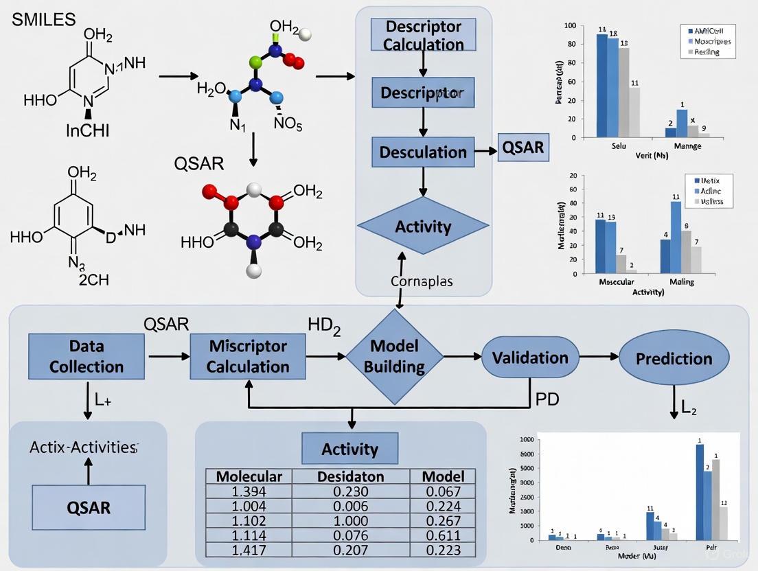
The development of a robust, predictive QSAR model follows a systematic workflow, from data curation to final validation. Adherence to this workflow is critical for regulatory acceptance, particularly under frameworks like the OECD principles [11].

The Standard QSAR Modeling Workflow

The following diagram illustrates the standard workflow for building a validated QSAR model.

Data Preparation and Molecular Representations

The initial and most critical phase involves the careful preparation of input data.

• Dataset Collection: A dataset of chemical structures and associated biological activities (e.g., IC₅₀, Ki) is compiled from reliable sources like ChEMBL or DrugBank [10] [16]. The dataset must be of high quality, with standardized biological values and curated structures.
• Data Cleaning and Preprocessing: This involves removing duplicates, standardizing structures (e.g., neutralizing charges, removing salts), handling missing values, and normalizing biological activity data (e.g., log-transformation) [10].
• Molecular Descriptor Calculation: Molecules are translated into numerical representations using software tools such as RDKit, Dragon, or PaDEL-Descriptor [17] [10]. Descriptors can be constitutional, topological, geometric, or electronic in nature [10].
• Feature Selection: Given the high dimensionality of descriptor spaces (often thousands of descriptors), techniques like random forest feature importance, LASSO regression, or mutual information filtering are employed to select the most relevant features and mitigate overfitting [17].

Model Building and Validation Protocols

This phase involves selecting algorithms, training models, and rigorously assessing their predictive power.

• Algorithm Selection: A spectrum of algorithms is used, ranging from interpretable linear models like Multiple Linear Regression (MLR) and Partial Least Squares (PLS) to non-linear methods like Support Vector Machines (SVM), Random Forests, and advanced deep learning architectures like Graph Neural Networks (GNNs) [15] [10] [16].
• Training and Validation: The dataset is split into training, validation, and external test sets. The model is built on the training set, and its hyperparameters are tuned using the validation set, often via k-fold cross-validation [10].
• External Validation and Applicability Domain: The final model's performance is assessed on a completely held-out external test set. Furthermore, the applicability domain (AD) must be defined to identify the chemical space within which the model can make reliable predictions [11] [16]. This is a key requirement for regulatory acceptance [11].

Table 2: Summary of Common QSAR Modeling Algorithms and Their Applications

Algorithm Category	Specific Examples	Typical Applications	Key Advantages & Limitations
Linear Methods	Multiple Linear Regression (MLR), Partial Least Squares (PLS) [10] [16]	Establishing baseline models; interpretable relationships [16]	Advantages: High interpretability, simple to implement.Limitations: Assumes linearity, cannot capture complex interactions.
Non-Linear Machine Learning	Support Vector Machines (SVM), Random Forest (RF), Gradient Boosting [17] [10] [13]	Predictive toxicology, activity classification in complex datasets [13]	Advantages: Captures non-linear relationships, generally good performance.Limitations: Can be prone to overfitting; less interpretable than linear models.
Deep Learning	Graph Neural Networks (GNNs), Multi-Layer Perceptrons (MLPs), Transformers [15] [17] [13]	State-of-the-art activity prediction; direct learning from molecular graphs or SMILES [15]	Advantages: State-of-the-art accuracy; automatic feature learning.Limitations: "Black-box" nature; requires large datasets and computational resources.

Contemporary Innovations and Future Directions

The field of QSAR is undergoing a rapid transformation driven by AI, leading to novel modeling paradigms that enhance both predictive power and integrative capacity.

Graph Neural Networks and Multi-Modal Learning

A significant advancement is the application of Graph Neural Networks (GNNs), which natively operate on molecular graphs where atoms are nodes and bonds are edges [15]. This representation allows GNNs to learn rich, hierarchical features directly from the molecular structure, often outperforming traditional models that rely on pre-defined fingerprints [15] [13]. Furthermore, multi-modal learning frameworks (e.g., Uni-QSAR) are being developed to integrate diverse data types, such as 1D SMILES sequences, 2D molecular graphs, and 3D spatial conformations, within a single model, leading to more robust predictions [17].

Explainable AI and Federated Learning

To address the "black-box" nature of complex AI models, Explainable AI (XAI) techniques are being incorporated to provide insights into the model's decision-making process, enhancing trust and interpretability for experimental validation teams [12]. Simultaneously, federated learning frameworks are emerging as a solution to data privacy challenges, allowing for the decentralized training of models across multiple institutions without sharing proprietary data [12].

Emerging Quantum and Hybrid Approaches

On the horizon, quantum machine learning (QML) is being explored for QSAR. Early studies suggest that quantum-enhanced kernel methods can outperform classical counterparts in limited-data settings, potentially opening new avenues for modeling complex structure-activity landscapes [17].

The following diagram illustrates how these modern approaches create an integrated, AI-driven QSAR workflow.

For researchers embarking on QSAR modeling, a suite of software tools and data resources is essential. The following table details key components of the modern QSAR toolkit.

Table 3: Essential Research Reagents and Resources for QSAR Modeling

Resource Category	Specific Tools / Databases	Primary Function in QSAR Workflow
Descriptor Calculation	RDKit, Dragon, PaDEL-Descriptor, Mordred [17] [10]	Generates numerical molecular descriptors from chemical structures for model training.
Chemical Databases	ChEMBL, ZINC, PubChem, DrugBank [12] [10]	Provides access to millions of compounds with annotated bioactivity data for dataset building.
Machine Learning Libraries	Scikit-learn, DeepChem, Keras, PyTorch, DGL [15] [17] [13]	Offers implementations of classic and deep learning algorithms for model construction.
Toxicology Data	Tox21 Challenge Data [15] [13]	Supplies standardized experimental screening results for training predictive toxicology models.
Validation & Compliance	OECD QSAR Toolbox [11]	Aids in following OECD validation principles for regulatory submission.

The journey of QSAR from the foundational equation of Crum-Brown and Fraser to the contemporary AI-powered models illustrates a remarkable evolution in computational chemistry. The field has matured from establishing simple linear relationships based on a handful of physicochemical parameters to leveraging deep learning on complex molecular graphs. The future of QSAR lies not in the replacement of traditional methods, but in their intelligent integration with contemporary AI, creating hybrid models that are both powerful and interpretable [12]. As these models become more sophisticated through the incorporation of explainable AI, federated learning, and multi-modal data, they are poised to further accelerate drug discovery, refine toxicity assessments, and contribute significantly to the development of safer, more effective therapeutics. For the scientific community, mastering both the historical foundations and the modern innovations outlined in this guide is essential for advancing research in computational medicinal chemistry.

Quantitative Structure-Activity Relationship (QSAR) models are regression or classification models used in chemical and biological sciences to relate a set of "predictor" variables to the potency of a response variable, which is typically a biological activity of chemicals [18]. The fundamental assumption underlying all QSAR approaches is that similar molecules have similar activities, a principle formally known as the Structure-Activity Relationship (SAR) [18]. In practice, QSAR modeling translates this principle into a mathematical framework where biological activity is expressed as a function of physicochemical properties and/or structural properties plus an error term: Activity = f(physiochemical properties and/or structural properties) + error [18].

The development of reliable QSAR models depends critically on three essential components: high-quality datasets, precisely calculated molecular descriptors, and appropriate mathematical models [19]. Molecular descriptors serve as the fundamental bridge between chemical structure and predicted activity—they are mathematical representations that quantify various electronic, geometric, or steric properties of molecules [20] [18]. By converting structural information into numerical values, descriptors enable the application of statistical and machine learning methods to find correlations between molecular structure and biological response. The accuracy and relevance of these descriptors directly determine the predictive power and interpretability of the resulting QSAR models [19].

Classification of Molecular Descriptors

Molecular descriptors can be categorized based on the dimensionality of the structural information they encode and the specific properties they represent. The diagram below illustrates the hierarchical classification of major descriptor types and the QSAR modeling approaches they enable.

Figure 1: Classification of molecular descriptors and their associated QSAR approaches.

One-Dimensional (1D) Descriptors

1D descriptors, also known as bulk properties, represent whole-molecule characteristics without considering atomic connectivity or three-dimensional geometry. These include fundamental physicochemical properties such as the octanol-water partition coefficient (logP), which measures lipophilicity; molar refractivity (MR), which combines molecular size and polarizability; and various other thermodynamic parameters [18]. In classical QSAR approaches like Hansch analysis, these global properties are correlated with biological activity under the assumption that absorption, distribution, and binding interactions can be captured through such macroscopic properties [19].

Two-Dimensional (2D) Descriptors

2D descriptors are derived from the molecular graph structure, considering atomic connectivity but ignoring three-dimensional conformation. This category includes topological indices that encode information about molecular branching, size, and shape based on graph theory representations [18]. Also belonging to this category are electronic descriptors that quantify charge distribution, polarizability, and orbital characteristics. These descriptors can be computed directly from molecular connection tables and are particularly valuable for high-throughput screening and initial structure-activity analyses [19].

Three-Dimensional (3D) Descriptors

3D descriptors capture the spatial arrangement of atoms in a molecule, recognizing that molecular binding occurs in 3D and that biological receptors perceive ligands as shapes carrying complex force fields [21]. The most significant 3D descriptors are Molecular Interaction Fields (MIFs), which map steric, electrostatic, and other interaction energies around molecules using various chemical probes [21]. These fields form the foundation of 3D-QSAR techniques like CoMFA (Comparative Molecular Field Analysis) and CoMSIA (Comparative Molecular Similarity Indices Analysis), which statistically correlate spatial field variations with biological activity differences across compound series [18] [21].

Fragment-Based Descriptors

Fragment-based descriptors operate on the principle of group contribution methods, where molecular properties are estimated as the sum of contributions from constituent structural fragments [18]. For example, the partition coefficient (logP) can be predicted using fragment methods known as "CLogP" that have been shown to generally provide better predictions than atomic-based methods [18]. This approach, formalized as GQSAR, offers flexibility to study various molecular fragments of interest in relation to biological response variation, and can consider cross-term fragment descriptors to identify key fragment interactions [18].

Mathematical Foundations of QSAR

Fundamental Mathematical Relationships

The mathematical core of QSAR modeling establishes a quantitative relationship between molecular descriptors (X) and biological activity (Y). This relationship can be expressed in two primary forms:

• Regression Models: For continuous activity values (e.g., IC₅₀, Ki), where Y = f(X) + ε
• Classification Models: For categorical activity outcomes (e.g., active/inactive, toxic/non-toxic) [18]

The transformation of biological activity data into appropriate mathematical representations is crucial. For binding affinities, values are typically converted to pIC₅₀ = -log₁₀(IC₅₀(M)) or pKi = -log₁₀(Ki(M)) to create linear relationships with free energy changes [22]. Activity thresholds are often applied for classification models, such as using 1 μM as a cutoff between active and inactive compounds [22].

Statistical and Machine Learning Methods

QSAR modeling employs diverse mathematical techniques, ranging from traditional statistical methods to advanced machine learning algorithms:

• Partial Least Squares (PLS): Particularly dominant in 3D-QSAR for handling the high dimensionality and multicollinearity of field descriptors [18] [21]
• Artificial Neural Networks (ANNs): Including specialized architectures like Counter-Propagation Artificial Neural Networks (CPANN) that can adaptively weight molecular descriptor importance during training [20]
• Support Vector Machines (SVM): Effective for both regression and classification tasks in chemical descriptor-based QSAR [18]
• Deep Learning Models: Emerging approaches that automatically learn relevant features from molecular structures without relying exclusively on pre-defined descriptors [19]

The mathematical model serves as the bridge between molecular structure and activity, with more flexible models capable of capturing complex, non-linear relationships but often at the cost of interpretability [19].

Quantitative Analysis of Descriptor Performance

Table 1: Performance comparison of qualitative vs. quantitative (Q)SAR models for antitarget prediction

Model Type	Balanced Accuracy	Sensitivity	Specificity	Compounds within Applicability Domain
Qualitative SAR (Ki values)	0.80	Generally higher	Lower	Higher
Quantitative QSAR (Ki values)	0.73	Generally lower	Higher	Lower
Qualitative SAR (IC₅₀ values)	0.81	Generally higher	Lower	Higher
Quantitative QSAR (IC₅₀ values)	0.76	Generally lower	Higher	Lower

Data derived from a study creating (Q)SAR models for 30 antitargets using GUSAR software and ChEMBL 20 database [22].

Table 2: Recent trends in QSAR research based on bibliometric analysis (2014-2023)

Research Aspect	Evolutionary Trend	Implications
Dataset Sizes	Steady increase	Enables more robust and generalizable models
Descriptor Types	Growing diversity with emphasis on 3D descriptors	Improved representation of molecular interactions
Model Complexity	Shift toward deep learning methods	Enhanced predictive ability but reduced interpretability
Model Validation	Increased focus on applicability domain assessment	Improved reliability for practical applications

Analysis based on publications in the Journal of Chemical Information and Modeling [19].

Experimental Protocols in QSAR Development

Data Set Preparation and Curation Protocol

• Data Extraction: Collect structures and experimental values (Ki, IC₅₀) from reliable databases like ChEMBL, ensuring consistent measurement units (nM) and relationship types (use only records with "=" in the "Relation" field) [22].

• Data Transformation: Convert activity values to pIC₅₀ = -log₁₀(IC₅₀(M)) or pKi = -log₁₀(Ki(M)) to establish linear relationships with free energy changes [22].

• Value Consolidation: For compounds with multiple experimental values, calculate median values to characterize strongly skewed distributions while retaining important chemical space coverage [22].

• Activity Thresholding: For classification models, establish thresholds between active and inactive compounds (e.g., 1 μM) [22].

• Data Splitting: Implement fivefold cross-validation by sorting sets by ascending activity values, assigning numbers 1-5 sequentially to structures, and dividing into five unique parts for training and testing [22].

Molecular Descriptor Calculation Methodology

• Descriptor Selection: Choose appropriate descriptors based on the QSAR approach (1D, 2D, 3D, or fragment-based) and the specific biological endpoint [19].

• 3D Structure Preparation: For 3D-QSAR, generate low-energy conformations and ensure proper alignment of training set compounds using crystallographic data or molecular superimposition software [21].

• Molecular Interaction Field Calculation:

  • Grid Generation: Superimpose a 3D lattice defining regularly distributed grid points around the molecules [21]
  • Probe Selection: Choose appropriate probes (carbon sp³ for steric fields, charged carbon sp³ for electrostatic fields, or multi-atom probes for specific interactions) [21]
  • Field Computation: Calculate interaction energies at each grid point using potential functions (Coulomb's law for electrostatic fields, Lennard-Jones potential for steric fields) [21]

• Descriptor Optimization: Apply feature selection techniques to reduce dimensionality while retaining chemically relevant information [19].

Model Validation and Applicability Domain Assessment

• Internal Validation: Perform cross-validation (e.g., fivefold CV) to assess model robustness [18].

• External Validation: Split data into training and prediction sets, or use blind external validation on new data [18].

• Statistical Analysis: Calculate correlation coefficients (R²), root mean square error (RMSE), balanced accuracy, sensitivity, and specificity [22] [18].

• Applicability Domain Definition: Establish the chemical space region where reliable predictions can be expected using approaches such as visual validation with tools like MolCompass, which employs parametric t-SNE models to visualize chemical space and identify model cliffs [23].

• Chance Correlation Testing: Perform Y-scrambling to verify absence of fortuitous correlations [18].

Table 3: Essential computational tools and resources for QSAR modeling

Tool/Resource	Type	Primary Function	Key Features
GUSAR Software	Software Platform	QSAR Model Development	Uses QNA and MNA descriptors; self-consistent regression [22]
ChEMBL Database	Chemical Database	Bioactivity Data Source	Manually curated data on drug-like molecules and their biological effects [22]
GRID Program	Computational Tool	Molecular Interaction Field Calculation	Multiple probes for mapping interaction energies in active sites [21]
VEGA Platform	QSAR Tool	Environmental Fate Prediction	Multiple models for persistence, bioaccumulation, and mobility [24]
MolCompass	Visualization Framework	Chemical Space Navigation	Parametric t-SNE for visual validation of QSAR models [23]
CPANN Algorithms	Modeling Algorithm	Neural Network QSAR	Adaptive descriptor importance weighting; interpretable models [20]

Advanced Concepts and Future Directions

Interpretability and Mechanistic Insight

A significant challenge in modern QSAR modeling lies in balancing predictive accuracy with interpretability. The Organisation for Economic Co-operation and Development (OECD) emphasizes the importance of "a mechanistic interpretation, if possible" as one of its key principles for QSAR validation [20]. Advanced approaches like the modified Counter-Propagation Artificial Neural Networks (CPANN) dynamically adjust molecular descriptor importance during training, allowing identification of key molecular features responsible for classifying molecules into specific endpoint classes [20]. This capability bridges the gap between "black box" predictions and chemically meaningful insights, potentially revealing relationships between selected molecular descriptors and known structural alerts for toxicity or other endpoints [20].

Expanding the Applicability Domain

The applicability domain (AD) represents the chemical space region where a QSAR model can reliably predict activity, and its proper definition remains crucial for trustworthy predictions [23]. Recent approaches focus on visual validation of QSAR models, enabling researchers to identify compounds or regions of chemical space where model predictions are unsatisfactory [23]. Tools like MolCompass implement parametric t-SNE models to create deterministic projections of chemical space, allowing consistent mapping of new compounds and facilitating identification of "model cliffs" where small structural changes lead to large prediction errors [23]. This visualization approach complements numerical AD metrics and enhances understanding of model limitations.

Emerging Trends and Universal QSAR Goals

The pursuit of universally applicable QSAR models capable of reliably predicting properties/activities across diverse chemical spaces continues to drive methodological innovations. Bibliometric analyses reveal several emerging trends, including the development of larger and higher-quality datasets, more accurate molecular descriptors, and the integration of deep learning methods that automatically learn relevant features from molecular structures [19]. The ongoing challenge lies in addressing three fundamental requirements: (1) sufficient training data to cope with molecular complexity and diversity, (2) precise molecular descriptors that balance dimensionality and computational cost, and (3) powerful yet flexible mathematical models capable of learning complex structure-activity relationships [19]. As these elements continue to evolve, the predictive ability, interpretability, and application domain of QSAR models will continue to expand, solidifying their role as indispensable tools in molecular design and drug discovery.

The Crucial Role of QSAR in Modern Drug Discovery and Development

Quantitative Structure-Activity Relationship (QSAR) modeling represents a cornerstone of modern computational drug discovery, enabling researchers to mathematically correlate the chemical structures of compounds with their biological activities. The foundational principle of QSAR—that a molecule's biological activity is determined by its molecular structure—has transformed pharmaceutical development from a largely empirical process to a rational, data-driven science [25]. Over the past six decades, QSAR has evolved from simple linear models based on a few physicochemical parameters to sophisticated artificial intelligence (AI)-driven approaches capable of navigating complex chemical spaces [19]. This evolution has positioned QSAR as an indispensable tool for addressing the formidable challenges of contemporary drug development, where escalating costs (exceeding $2.8 billion per approved drug), extended timelines (10-15 years), and high failure rates necessitate more efficient and predictive approaches [16].

The integration of QSAR methodologies into drug discovery pipelines provides a strategic framework for prioritizing chemical synthesis and experimental testing, significantly reducing resource burdens while increasing the probability of success. By enabling the virtual screening of large compound libraries, QSAR models allow researchers to focus experimental efforts on the most promising candidates, thereby compressing discovery timelines and reducing reliance on extensive animal testing [26]. In today's era of AI-enabled drug discovery, QSAR has emerged as a platform technology that synergizes with structural biology, cheminformatics, and machine learning to accelerate the identification and optimization of therapeutic compounds across diverse disease areas [27] [28].

Theoretical Foundations and Methodological Evolution

Historical Development and Basic Principles

The conceptual origins of QSAR trace back to the 19th century when Crum-Brown and Fraser first proposed that the physiological activity of molecules depends on their chemical structure [16]. The field formally began in the early 1960s with the pioneering work of Hansch and Fujita, who developed a method for predicting biological activity using physicochemical parameters such as lipophilicity (log P), electronic properties (Hammett constants), and steric effects [25]. This approach, known as Hansch analysis, established the fundamental QSAR paradigm of expressing biological activity as a mathematical function of molecular descriptors:

Activity = f(D₁, D₂, D₃...) where D₁, D₂, D₃ represent molecular descriptors [16].

The underlying principle of similarity states that compounds with similar structures tend to exhibit similar biological activities, forming the basis for predicting properties of novel compounds based on their position in chemical space [25]. This principle enables QSAR models to generalize from known structure-activity relationships to new chemical entities, providing a powerful framework for molecular design.

The QSAR Workflow: From Data Curation to Model Validation

The development of reliable QSAR models follows a systematic workflow comprising several critical stages, each requiring rigorous execution to ensure predictive accuracy and relevance.

Figure 1: Comprehensive QSAR modeling workflow illustrating the sequential stages from data collection to predictive application.

The process begins with the collection and curation of high-quality datasets containing chemical structures and corresponding biological activities (e.g., IC₅₀, EC₅₀ values) obtained through standardized experimental protocols [16] [19]. Data curation is particularly critical, as chemical structure errors directly propagate to model inaccuracies [27]. The next stage involves molecular descriptor calculation, where chemical structures are translated into numerical representations encoding various physicochemical, topological, or quantum-chemical properties [19]. With thousands of potential descriptors available, feature selection and dimensionality reduction techniques such as Principal Component Analysis (PCA), Recursive Feature Elimination (RFE), or LASSO regularization are employed to identify the most relevant descriptors and mitigate overfitting [28] [19].

Model development applies statistical or machine learning algorithms to establish mathematical relationships between selected descriptors and biological activity. This stage typically utilizes a training set of compounds (approximately 75-80% of available data) to build the model [29]. Finally, rigorous validation assesses model performance on external test sets and defines the applicability domain—the chemical space within which the model provides reliable predictions [16] [19]. The leverage method is commonly used to determine this domain, ensuring that predictions are only made for compounds structurally similar to those in the training set [16].

Molecular Descriptors: Encoding Chemical Information

Molecular descriptors serve as the fundamental building blocks of QSAR models, quantitatively representing specific aspects of molecular structure and properties. These descriptors are typically categorized based on the complexity of structural information they encode:

Table 1: Classification of Molecular Descriptors in QSAR Modeling

Descriptor Type	Description	Examples	Applications
1D Descriptors	Global molecular properties	Molecular weight, log P (partition coefficient), pKa	Preliminary screening, physicochemical property prediction
2D Descriptors	Topological descriptors based on molecular connectivity	Molecular fingerprints, topological indices, graph-based descriptors	Similarity searching, large-scale virtual screening
3D Descriptors	Spatial molecular features	Molecular surface area, volume, steric parameters, electrostatic potentials	Structure-based design, conformational analysis
4D Descriptors	Conformational ensembles accounting for flexibility	Multiple molecular conformations, interaction fields	Pharmacophore modeling, receptor-based design
Quantum Chemical Descriptors	Electronic structure properties	HOMO-LUMO energies, dipole moment, electrostatic potential surfaces	Mechanism analysis, reactivity prediction

Recent advances include "deep descriptors" derived from neural networks that automatically learn relevant molecular features from raw structural data such as SMILES strings or molecular graphs, potentially capturing more complex structure-activity relationships than traditional engineered descriptors [28].

Classical to Modern: The Evolution of QSAR Modeling Techniques

Classical Statistical Approaches

Classical QSAR methodologies rely on statistical techniques to establish linear relationships between molecular descriptors and biological activity. These methods remain valuable for their interpretability and robustness, particularly with limited datasets.

Multiple Linear Regression (MLR) represents one of the most widely used classical approaches, generating models in the form of simple linear equations that are easily interpretable [16] [28]. Partial Least Squares (PLS) regression excels in handling datasets with numerous correlated descriptors by projecting variables into a lower-dimensional space of latent factors [28]. Principal Component Regression (PCR) combines PCA with regression, using principal components as independent variables to address multicollinearity issues [28].

The primary limitation of classical approaches lies in their assumption of linear relationships between descriptors and activity, which often fails to capture the complex, nonlinear interactions prevalent in biological systems. Additionally, these methods typically require careful feature selection to avoid overfitting and maintain model interpretability [28].

Machine Learning and Ensemble Methods

Machine learning has dramatically expanded the capabilities of QSAR modeling by enabling the detection of complex, nonlinear patterns in high-dimensional chemical data. These algorithms automatically learn the relationship between molecular structure and biological activity without pre-specified assumptions about the underlying functional form.

Table 2: Machine Learning Algorithms in QSAR Modeling

Algorithm	Principles	Advantages	Limitations
Random Forest (RF)	Ensemble of decision trees using bagging	Handles noisy data, built-in feature selection, robust to outliers	Limited extrapolation beyond training data
Support Vector Machines (SVM)	Finds optimal hyperplane to separate classes	Effective in high-dimensional spaces, memory efficient	Performance depends on kernel selection
k-Nearest Neighbors (kNN)	Predicts based on similar compounds in descriptor space	Simple implementation, no training phase	Computationally intensive for large datasets
Artificial Neural Networks (ANN)	Network of interconnected nodes mimicking neural processing	Captures complex nonlinear relationships, handles diverse data types	Requires large datasets, prone to overfitting

Ensemble methods have emerged as particularly powerful approaches, combining multiple models to produce more accurate and stable predictions than any single constituent model. Comprehensive ensemble techniques that diversify across multiple subjects (different algorithms, descriptor types, and data splits) have demonstrated superior performance compared to individual models or limited ensembles [29]. For example, a comprehensive ensemble method applied to 19 bioassay datasets achieved an average AUC of 0.814, outperforming individual models like ECFP-RF (AUC 0.798) and PubChem-RF (AUC 0.794) [29].

Deep Learning and the Emergence of Deep QSAR

The integration of deep learning represents the cutting edge of QSAR modeling, giving rise to the subfield of "deep QSAR" [27]. Deep neural networks with sophisticated architectures can automatically learn hierarchical molecular representations directly from structural data, eliminating the need for manual descriptor engineering.

Graph Neural Networks (GNNs) operate directly on molecular graphs, treating atoms as nodes and bonds as edges, thereby naturally representing molecular topology [27] [28]. SMILES-based transformers adapt natural language processing techniques to process simplified molecular input line entry system strings as chemical "sentences" [27]. Convolutional Neural Networks (CNNs) applied to molecular structures can detect spatially localized structural patterns relevant to biological activity [29].

These deep learning approaches demonstrate particular strength in scenarios with large, diverse chemical datasets, where they can uncover complex structure-activity relationships that elude traditional methods. The ANN [8.11.11.1] architecture applied to NF-κB inhibitors, for instance, demonstrated superior reliability and predictive power compared to MLR models [16].

Experimental Protocols and Implementation Frameworks

Protocol: Development and Validation of a QSAR Model for NF-κB Inhibitors

The following detailed protocol exemplifies a robust QSAR modeling approach, as applied to Nuclear Factor-κB (NF-κB) inhibitors, a promising therapeutic target for immunoinflammatory diseases and cancer [16]:

• Dataset Compilation:

  • Curate 121 compounds with reported experimental IC₅₀ values against NF-κB from literature sources
  • Ensure consistent activity measurements obtained through standardized bioassays
  • Apply chemical structure standardization and curation to eliminate errors

• Data Division:

  • Randomly partition compounds into training (~66%) and test sets (~34%)
  • Maintain similar activity distributions across both sets
  • Apply the leverage method to define the applicability domain

• Descriptor Calculation and Selection:

  • Compute molecular descriptors using cheminformatics software (e.g., DRAGON, PaDEL, RDKit)
  • Apply ANOVA for initial descriptor screening based on statistical significance
  • Utilize correlation analysis and stepwise selection to identify optimal descriptor subsets

• Model Development:

  • Implement MLR with feature selection to generate linear models
  • Train ANN architectures (e.g., [8.11.11.1] topology) using backpropagation
  • Apply regularization techniques (e.g., weight decay, dropout) to prevent overfitting

• Model Validation:

  • Perform internal validation using 5-fold cross-validation on training set
  • Conduct external validation using held-out test set
  • Calculate statistical metrics: R² (coefficient of determination), Q² (cross-validated R²), RMSE (root mean square error)
  • Apply Y-randomization to confirm model robustness

• Model Interpretation and Application:

  • Analyze descriptor contributions to identify structural features influencing activity
  • Utilize the validated model to predict activities of novel compounds
  • Synthesize and test highest-ranking candidates for experimental verification

Successful QSAR modeling relies on specialized software tools, databases, and computational resources that collectively enable the construction and application of predictive models.

Table 3: Essential Resources for QSAR Modeling

Resource Category	Specific Tools	Function	Availability
Cheminformatics Software	RDKit, PaDEL-Descriptor, DRAGON	Molecular descriptor calculation, structural analysis	Open-source / Commercial
QSAR Modeling Platforms	QSARINS, KNIME, Scikit-learn	Model development, validation, and visualization	Open-source / Commercial
Chemical Databases	PubChem, ChEMBL, ZINC	Source of chemical structures and bioactivity data	Publicly accessible
Molecular Visualization	PyMOL, Chimera, MarvinView	Structure manipulation and analysis	Freemium / Commercial
Programming Environments	Python, R, Julia	Custom model implementation and analysis	Open-source

Applications in Contemporary Drug Discovery

Target-Based Drug Discovery

QSAR models have become integral to targeted drug discovery campaigns against specific therapeutic targets. In anti-breast cancer drug development, QSAR has been extensively applied to optimize compounds targeting estrogen receptors, HER2, and various kinase pathways [25]. Similarly, for Alzheimer's disease, researchers have developed 2D-QSAR models to design blood-brain barrier permeable BACE-1 inhibitors, successfully optimizing key molecular properties while maintaining potency [28].

In antiviral discovery, QSAR approaches have been deployed against SARS-CoV-2 targets, with machine learning models developed to screen potential main protease (Mᴾʳᵒ) inhibitors, rapidly identifying candidate compounds for experimental validation [28]. These target-specific applications demonstrate how QSAR accelerates lead optimization by providing clear design rules that mediate the trade-offs between potency, selectivity, and physicochemical properties.

ADMET Prediction and Toxicity Assessment

Beyond primary pharmacology, QSAR models have become indispensable tools for predicting absorption, distribution, metabolism, excretion, and toxicity (ADMET) properties early in the drug discovery process. These applications directly address the high attrition rates in drug development, where pharmacokinetic and safety issues remain leading causes of failure [26] [28].

Environmental toxicology represents another significant application area, where QSAR models predict the ecotoxicological effects of chemicals on various species, supporting regulatory decisions and green chemistry initiatives [26]. The implementation of QSAR in regulatory contexts, such as the REACH framework in Europe, highlights the maturity and reliability of well-validated models for specific endpoints [28].

Emerging Applications: PROTACs and Targeted Protein Degradation

QSAR modeling is expanding into novel therapeutic modalities, most notably proteolysis-targeting chimeras (PROTACs) and other targeted protein degradation approaches [28]. These heterobifunctional molecules present unique modeling challenges due to their larger size, complex physicochemical properties, and dual-target engagement requirements. QSAR approaches adapted for these degraders must account for ternary complex formation, cellular permeability challenges, and hook effect dynamics—representing an exciting frontier for methodological innovation [28].

Current Trends and Future Perspectives

AI Integration and Multidisciplinary Convergence

The integration of artificial intelligence with QSAR modeling continues to advance, with several emerging trends shaping the field's trajectory. Explainable AI approaches, including SHAP (SHapley Additive exPlanations) and LIME (Local Interpretable Model-agnostic Explanations), are addressing the "black box" problem of complex models by providing mechanistic insights into predictions [28]. Multi-task learning frameworks simultaneously model multiple biological endpoints, leveraging shared information to improve generalization, particularly for datasets with limited compounds [27] [29].

The field is also witnessing increased multidisciplinary integration, with QSAR serving as a bridge between computational chemistry, structural biology, and systems pharmacology [30]. This convergence enables the development of more physiologically relevant models that incorporate target engagement data from technologies like Cellular Thermal Shift Assay (CETSA) to validate computational predictions in biologically complex systems [30].

Quantum Computing and Next-Generation QSAR

Quantum computing represents a frontier technology with potential applications in QSAR modeling, particularly through Quantum Support Vector Machines (QSVMs) that leverage quantum mechanical principles to process information in Hilbert spaces [31] [32]. These approaches theoretically offer advantages for handling high-dimensional data and capturing complex molecular interactions, though they remain in early developmental stages [31].

Challenges and Implementation Considerations

Despite substantial advances, QSAR modeling faces several persistent challenges. Data quality and standardization remain critical, as model performance is fundamentally limited by the quality of training data [27] [19]. Model interpretability becomes increasingly difficult with complex deep learning architectures, creating barriers to chemical intuition and design [28]. Applicability domain characterization requires careful attention to ensure models are not applied beyond their validated chemical spaces [16] [19].

Successful implementation requires rigorous validation protocols, domain awareness, and integration with experimental verification in iterative design-make-test-analyze cycles. As the field progresses, the development of universal QSAR models capable of accurate predictions across diverse chemical spaces remains an aspirational goal—one that will require advances in dataset size and quality, molecular representation, and algorithm development [19].

QSAR modeling has evolved from its origins in linear regression to become an indispensable component of modern drug discovery, integrated throughout the value chain from target validation to lead optimization. The convergence of QSAR with artificial intelligence, structural biology, and experimental pharmacology has created a powerful ecosystem for accelerated therapeutic development. As methodological innovations continue to emerge—particularly in deep learning, explainable AI, and quantum-inspired algorithms—QSAR's predictive power and domain of applicability will continue to expand. For researchers and drug development professionals, mastery of QSAR principles and applications represents not merely a technical skill but a strategic imperative in the quest to develop novel therapeutics with greater efficiency and success.

Quantitative Structure-Activity Relationship (QSAR) modeling represents a cornerstone of modern computational chemistry and drug discovery, providing mathematical frameworks that correlate chemical structure with biological activity or physicochemical properties [18]. These models are founded on the fundamental principle that the structure of a molecule determines its properties, enabling researchers to predict the activity of new compounds without costly and time-consuming synthetic effort and biological testing [33]. The general form of a QSAR model is expressed as Activity = f(physicochemical properties and/or structural properties) + error, where the function relates molecular descriptors to a quantitative measure of biological response [18]. The evolution of QSAR methodologies has progressed through distinct generations characterized by increasing sophistication in molecular representation—from simple atomic counts to complex conformational ensembles—each building upon the limitations of its predecessor to offer more accurate and mechanistically insightful predictions [34] [28].

The predictive power of QSAR models has made them indispensable across multiple scientific disciplines, including drug discovery, toxicology, environmental science, and materials science [18] [33]. In pharmaceutical research specifically, QSAR approaches have transitioned from traditional statistical models to advanced machine learning and deep learning frameworks that can capture complex nonlinear relationships across expansive chemical spaces [28]. This technical guide examines the fundamental descriptor types that form the foundation of all QSAR modeling, categorized by their dimensional representation, and provides researchers with a comprehensive framework for selecting appropriate descriptors based on their specific research objectives.

Molecular Descriptors: The Foundation of QSAR

Molecular descriptors are quantifiable numerical representations that capture the structural, physicochemical, and biological properties of chemical compounds [34] [33]. These descriptors serve as the independent variables in QSAR models, encoding chemical information into a mathematical form suitable for statistical analysis and machine learning algorithms [28]. The process of transforming molecular structures into numerical descriptors enables the application of pattern recognition, regression techniques, and classification algorithms to predict biological activities and properties of untested compounds [34].

The concept of dimensionality in molecular descriptors refers to the level of structural representation used to compute them, ranging from simple atomic counts to complex representations that account for molecular flexibility and dynamics [33]. Higher-dimensional descriptors typically capture more complex structural information but require greater computational resources and more sophisticated modeling approaches [35]. The appropriate selection of descriptors is crucial for developing robust QSAR models, as it directly influences model accuracy, interpretability, and applicability domain [18] [33].

Table 1: Classification of Molecular Descriptors by Dimension

Descriptor Dimension	Structural Information Encoded	Example Descriptors	Common Applications
1D Descriptors	Global molecular properties derived from chemical formula	Molecular weight, atom counts, bond counts, logP [34] [33]	Preliminary screening, high-throughput profiling [33]
2D Descriptors	Structural connectivity and topology	Topological indices, connectivity indices, 2D fingerprints, molecular graphs [34] [33]	Virtual screening, similarity searching, toxicity prediction [34] [33]
3D Descriptors	Spatial molecular geometry and shape	Molecular surface area, volume, electrostatic potentials, steric fields [18] [36] [37]	Lead optimization, structure-based design [36] [37]
4D Descriptors	Conformational ensembles and dynamics	Interaction energy descriptors (Lennard-Jones, Coulomb), occupancy profiles [35] [38]	Modeling flexible molecules, protein-ligand interactions [35] [38]

The selection of appropriate descriptors must balance computational efficiency with representational completeness, while always considering the domain of applicability and the specific biological endpoint being modeled [18] [33]. As the pharmaceutical industry increasingly embraces AI-driven approaches, molecular descriptors continue to evolve, with graph-based representations and learned embeddings offering new opportunities for capturing complex structure-activity relationships [28].

1D Descriptors: One-Dimensional Representations

1D descriptors represent the most fundamental level of molecular representation, encoding global molecular properties that can be derived directly from the chemical formula or connection table without consideration of molecular geometry or topology [33]. These descriptors provide a coarse-grained characterization of molecules and are computationally efficient to calculate, making them suitable for initial screening and profiling of large chemical libraries [34]. Common 1D descriptors include molecular weight, element counts, ring counts, and the partition coefficient (LogP), which provides information about a compound's hydrophobicity [34] [33].

The primary advantage of 1D descriptors lies in their computational simplicity and ease of interpretation [33]. Models based on 1D descriptors typically train quickly and can provide initial structure-activity trends with minimal computational investment. However, this simplicity comes at the cost of limited structural resolution, as 1D descriptors contain no information about atomic connectivity or spatial arrangement [34]. Consequently, QSAR models based solely on 1D descriptors often lack the granularity needed for lead optimization stages in drug discovery, though they remain valuable for preliminary property profiling and high-throughput prioritization [33].

2D Descriptors: Two-Dimensional Representations

2D descriptors incorporate information about the connectivity of atoms within a molecule, representing the molecular structure as a graph where atoms correspond to vertices and bonds to edges [33]. This topological representation enables the calculation of descriptors that capture more nuanced structural patterns than is possible with 1D descriptors alone [34]. The most commonly used 2D descriptors include constitutional descriptors (representing molecular composition), electrostatic descriptors (reflecting electronic distribution), topological descriptors (derived from graph theory), and fragment-based descriptors that encode the presence of specific functional groups or substructures [33].

Topological descriptors, such as connectivity indices and molecular fingerprints, are particularly valuable for similarity searching and virtual screening [34]. Molecular fingerprints, including MDL keys and PubChem fingerprints, represent molecules as bit strings that indicate the presence or absence of specific structural features [33]. These descriptors enable rapid comparison of chemical structures across large databases and have become fundamental tools in chemoinformatics [34]. The widespread adoption of 2D descriptors stems from their favorable balance between computational efficiency and structural information content, making them the most commonly used descriptor type in QSAR modeling [33].

Table 2: Categories and Examples of 2D Molecular Descriptors

Descriptor Category	Description	Specific Examples
Constitutional Descriptors	Properties related to molecular composition	Molecular weight, total number of atoms, number of aromatic rings [33]
Topological Descriptors	Properties derived from molecular graph representation	Connectivity indices, Wiener index, Zagreb index [33]
Electrostatic Descriptors	Properties related to electronic distribution	Partial atomic charges, dipole moment, polarizability [33]
Geometrical Descriptors	Properties related to atomic spatial arrangement (calculated from 2D coordinates)	Van der Waals surface area, shadow indices [33]
Fragment-Based Descriptors	Presence or absence of specific structural motifs	Molecular fingerprints, MDL keys, functional group counts [33]

Despite their utility, 2D descriptors share a significant limitation with their 1D counterparts: they contain no explicit information about the three-dimensional conformation of molecules, which is often critical for biological recognition and activity [35]. This limitation becomes particularly important when modeling interactions with structurally defined biological targets, necessitating the use of higher-dimensional descriptors for more accurate activity prediction [36] [37].

3D Descriptors: Three-Dimensional Representations

3D descriptors encode information about the spatial arrangement of atoms in a molecule, providing a representation of molecular shape, steric bulk, and electronic distribution in three-dimensional space [18] [36]. These descriptors are typically derived from a single, low-energy conformation of a molecule or from an alignment of multiple molecules based on their putative binding mode [37]. The development of 3D-QSAR approaches, such as Comparative Molecular Field Analysis (CoMFA) and Comparative Molecular Similarity Indices Analysis (CoMSIA), represents a significant advancement in QSAR methodology by explicitly relating biological activity to interaction fields surrounding molecules [18] [36].

In 3D-QSAR studies, molecules are first aligned in three-dimensional space based on either experimental data (e.g., protein-ligand crystal structures) or molecular superimposition algorithms [18]. Interaction fields, including steric (shape) and electrostatic potentials, are then calculated at grid points surrounding the aligned molecules [36]. These interaction potentials serve as the 3D descriptors in the QSAR model, which is typically constructed using partial least squares (PLS) regression to handle the high dimensionality of the descriptor space [18] [36]. The resulting models provide visual representations of regions in space where specific molecular properties enhance or diminish biological activity, offering medicinal chemists intuitive guidance for structural modification [36].

A recent application of 3D-QSAR modeling demonstrated its continued relevance in modern drug discovery. In a study on 6-hydroxybenzothiazole-2-carboxamide derivatives as monoamine oxidase B (MAO-B) inhibitors, researchers developed a CoMSIA model with excellent predictive ability (q² = 0.569, r² = 0.915) [36]. The model successfully identified key structural features influencing MAO-B inhibition and guided the design of novel derivatives with predicted nanomolar activity, subsequently validated through molecular docking and dynamics simulations [36]. Similarly, a 3D-QSAR study on indole derivatives as aromatase inhibitors for breast cancer treatment employed a Self-Organizing Molecular Field Analysis (SOMFA) approach, effectively predicting activity using shape and electrostatic potential fields [37].

Figure 1: The typical workflow for 3D-QSAR model development, involving conformation generation, molecular alignment, field calculation, and model validation.

Despite their advantages in capturing spatial properties, 3D-QSAR methods have limitations, particularly their dependence on molecular alignment and their treatment of molecules as rigid entities with single, bioactive conformations [35]. This simplification fails to account for the dynamic nature of ligand-receptor interactions, where both partners exhibit conformational flexibility [35] [38]. This limitation has motivated the development of more advanced four-dimensional QSAR approaches that explicitly incorporate molecular flexibility.

4D Descriptors: Four-Dimensional Representations

4D descriptors extend the concept of 3D-QSAR by incorporating molecular flexibility as the fourth dimension, representing molecules as ensembles of conformations, orientations, tautomers, or protonation states rather than single static structures [35] [38]. This approach acknowledges that molecules exist as dynamic ensembles under physiological conditions and that biological recognition often involves induced-fit mechanisms [38]. In 4D-QSAR, descriptors are computed as averages over multiple molecular states, providing a more realistic representation of the conformational space sampled by flexible molecules [35].

The fourth dimension in these descriptors typically refers to ensemble averaging of molecular states, addressing both conformational flexibility and alignment freedom that plague traditional 3D-QSAR methods [38]. Modern implementations of 4D-QSAR, such as the LQTA-QSAR method, use molecular dynamics (MD) simulations to generate conformational ensemble profiles (CEP) for each compound [38]. Interaction energy descriptors, including Lennard-Jones (LJ) and Coulomb (C) potentials, are computed from these ensembles and serve as the basis for model construction [38]. This MD-QSAR approach represents a significant advancement in the field, leveraging GPU-accelerated computing and modern machine learning techniques to handle the computational complexity of conformational sampling [35].

A recent application of 4D-QSAR to N-substituted urea/thioureas as human glutaminyl cyclase (hQC) inhibitors for Alzheimer's disease demonstrated the power of this approach [38]. The developed model showed excellent statistical reliability (Q² = 0.521, R² = 0.933) and successfully guided the design of new compounds with predicted enhanced activity [38]. Molecular dynamics simulations confirmed the stability of designed compounds in the hQC binding pocket, with several showing higher binding free energies than the reference compound [38]. This study exemplifies how 4D-QSAR can provide valuable insights for optimizing flexible molecules with complex structure-activity relationships.

Figure 2: 4D-QSAR workflow incorporating molecular dynamics simulations to account for conformational flexibility in descriptor calculation.

The resurgence of interest in 4D-QSAR, after a period of limited adoption due to computational constraints, reflects advances in simulation technologies and algorithmic efficiency [35]. The development of hyper-predictive MD-QSAR models has been described as a "disruptive technology" for analyzing and optimizing dynamic protein-ligand interactions, with countless applications in drug discovery and chemical toxicity assessment [35]. As computational resources continue to improve and machine learning approaches become more sophisticated, 4D-QSAR is poised to play an increasingly important role in rational drug design, particularly for challenging targets where flexibility plays a critical role in molecular recognition.

Experimental Protocols and Methodologies

3D-QSAR Protocol Using CoMSIA

The implementation of a robust 3D-QSAR study requires careful attention to each step of the modeling process. A representative protocol for CoMSIA analysis is outlined below, based on recent research investigating 6-hydroxybenzothiazole-2-carboxamide derivatives as MAO-B inhibitors [36]:

• Compound Selection and Preparation: Select a congeneric series of compounds with known biological activities spanning at least 3-4 orders of magnitude. Draw 2D structures using chemoinformatics software such as ChemDraw and convert to 3D structures using molecular modeling packages like Sybyl-X [36].

• Molecular Alignment: Superimpose molecules using a common scaffold or pharmacophoric features. The alignment should reflect putative binding modes, preferably guided by experimental structural data or molecular docking poses [36] [37].

• Interaction Field Calculation: Calculate steric, electrostatic, hydrophobic, and hydrogen-bonding fields at grid points surrounding the aligned molecules. The CoMSIA method typically uses a Gaussian function to avoid singularities at atomic positions [36].

• Partial Least Squares (PLS) Analysis: Construct the QSAR model using PLS regression to correlate interaction fields with biological activity. Implement leave-one-out or leave-group-out cross-validation to determine the optimal number of components and assess model robustness [36].

• Model Validation: Evaluate model performance using both internal validation (cross-validated correlation coefficient q²) and external validation (predictive correlation coefficient r²pred for an independent test set) [36] [33].

• Contour Map Analysis: Visualize the results as 3D contour maps indicating regions where specific molecular properties enhance or diminish biological activity. These maps provide intuitive guidance for structural optimization [36].

In the MAO-B inhibitor study, this protocol yielded a CoMSIA model with strong predictive ability (q² = 0.569, r² = 0.915, F = 52.714), successfully guiding the design of novel derivatives with improved predicted activity [36].

4D-QSAR Protocol Using LQTA-QSAR Method

The LQTA-QSAR approach incorporates molecular dynamics simulations to account for conformational flexibility. A typical protocol, as applied to N-substituted urea/thioureas as hQC inhibitors, includes the following steps [38]:

• Dataset Preparation: Curate a set of compounds with known biological activities. Randomly divide compounds into training and test sets, ensuring structural diversity and activity range representation in both sets [38].

• Conformational Sampling: Perform molecular dynamics simulations for each compound using software such as GROMACS. Generate conformational ensemble profiles (CEPs) through simulation in explicit solvent under physiological conditions [38].

• Descriptor Calculation: Compute interaction energy descriptors (Lennard-Jones and Coulomb potentials) for each conformation in the ensemble. Calculate ensemble-averaged descriptors to capture conformational flexibility [38].

• Model Construction: Build the 4D-QSAR model using partial least squares regression with the ensemble-averaged descriptors as independent variables and biological activity as the dependent variable [38].

• Model Validation: Validate the model using both internal (cross-validation) and external (test set prediction) methods. Additionally, perform randomization tests (Y-scrambling) to ensure the model does not result from chance correlation [38].

• Molecular Docking and Dynamics Validation: Supplement the 4D-QSAR analysis with molecular docking to visualize binding modes and molecular dynamics simulations to assess binding stability and interaction patterns [38].

This methodology produced a 4D-QSAR model for hQC inhibitors with satisfactory predictive ability (Q² = 0.521, R² = 0.933), enabling the design of new compounds with improved predicted binding affinities [38].

Table 3: Research Reagent Solutions for QSAR Modeling

Research Tool	Specific Examples	Primary Function	Availability
Cheminformatics Software	ChemDraw, BIOVIA Draw	2D structure drawing and 3D conversion	Commercial [36] [39]
Molecular Modeling Platforms	Sybyl-X, Discovery Studio	3D structure optimization, alignment, QSAR model development	Commercial [36] [39]
Descriptor Calculation Tools	DRAGON, PaDEL, RDKit	Computation of molecular descriptors from 0D to 3D	Commercial and Free [28] [33]
Dynamics Simulation Software	GROMACS, AMBER	Molecular dynamics simulations for 4D-QSAR	Free and Commercial [35] [38]
QSAR Modeling Programs	QSAR-KING, Build QSAR	Development and validation of QSAR models	Free and Commercial [38] [28]

Comparative Analysis and Research Applications

The selection of appropriate descriptor dimensions depends on multiple factors, including the research objective, computational resources, and nature of the structure-activity relationship under investigation [33]. 1D and 2D descriptors remain valuable for high-throughput screening and initial profiling of large compound libraries, where computational efficiency is paramount [34] [33]. These descriptors have proven particularly successful in virtual screening and toxicity prediction, where they can rapidly eliminate compounds with undesirable properties [33].

3D descriptors offer significant advantages when optimizing compounds for targets with known structural information or when molecular shape and electrostatic complementarity play critical roles in biological activity [36] [37]. The visual guidance provided by 3D-QSAR contour maps directly supports medicinal chemistry efforts by highlighting structural modifications likely to enhance potency [36]. However, the alignment dependence of these methods and their treatment of molecular rigidity represent significant limitations, particularly for flexible ligands [35].

4D descriptors address these limitations by explicitly incorporating molecular flexibility, making them particularly valuable for lead optimization stages where subtle conformational changes can significantly impact binding affinity [35] [38]. While computationally intensive, 4D-QSAR methods provide more realistic representations of ligand-receptor interactions and can model complex induced-fit binding mechanisms [38]. The recent resurgence of 4D-QSAR, driven by advances in GPU-accelerated computing and machine learning, promises to enhance our ability to design compounds for challenging biological targets with conformational flexibility [35].

In practical research applications, these descriptor types are often used complementarily rather than exclusively. A typical drug discovery pipeline might employ 2D descriptors for initial virtual screening, followed by 3D-QSAR for lead optimization, and 4D-QSAR for particularly challenging structure-activity relationships involving significant conformational flexibility [35] [28]. This multidimensional approach leverages the unique strengths of each descriptor type while mitigating their individual limitations.

The evolution of molecular descriptors from simple 1D representations to complex 4D ensembles mirrors the increasing sophistication of computational chemistry and its growing impact on drug discovery [28]. Each dimensional class offers distinct advantages and limitations, making them suited to different stages of the research pipeline and different types of structure-activity relationships [33]. As the field continues to advance, the integration of AI and machine learning with multidimensional QSAR approaches promises to further enhance predictive accuracy and mechanistic insight [28].

The resurgence of interest in 4D-QSAR, powered by advances in molecular dynamics simulations and machine learning, represents a particularly promising development for addressing the challenges of molecular flexibility in drug design [35] [38]. This evolution toward dynamic, ensemble-based representations acknowledges the inherent flexibility of both ligands and their biological targets, moving beyond the static view that has traditionally dominated molecular modeling [35]. For researchers seeking to implement QSAR methodologies, the selection of appropriate descriptor dimensions should be guided by the specific research question, available structural information, and computational resources, with the understanding that hybrid approaches often yield the most insightful results [28] [33].

As QSAR modeling continues to evolve, the integration of multidimensional descriptors with advanced machine learning algorithms, expanded chemical databases, and structural biology information will further blur the boundaries between traditional descriptor classifications [28]. This convergence promises to deliver increasingly accurate and interpretable models that accelerate the discovery of novel therapeutic agents and deepen our understanding of the molecular basis of biological activity [34] [28].

The QSAR Workflow in Action: Methodologies, Modeling, and Real-World Applications

The development of robust Quantitative Structure-Activity Relationship (QSAR) models is fundamentally dependent on the quality of the underlying chemical data [10]. These models mathematically link a chemical compound's structure to its biological activity or properties, operating on the principle that structural variations influence biological activity [10]. In modern computational chemistry, the advancement of machine learning and the availability of large chemical datasets have heightened interest in developing standardized tools and protocols [40]. The process transforms raw, often disparate, data into a clean, consistent, and reliable dataset suitable for computational analysis. For scientists and drug development professionals, rigorous data curation is not merely a preliminary step but a critical determinant of model predictivity, regulatory acceptance, and ultimately, the success of a drug discovery campaign [41] [10].

Data Collection and Consolidation

The initial phase involves gathering chemical structures and their associated biological activities from reliable sources. The goal is to compile a dataset that is both comprehensive and representative of the chemical space of interest [10].

Key Data Sources: Data can be retrieved from a combination of public databases and scientific literature.

• Public Databases: Sources such as ChEMBL, the EURL ECVAM Genotoxicity and Carcinogenicity dataset, and the Chemical Carcinogenesis Research Information System provide structured bioactivity data [41].
• Scientific Literature: Extracting data from peer-reviewed publications ensures access to the latest findings. To efficiently process the vast amount of published literature, advanced text-mining approaches are now being employed. For instance, one study used the BioBERT pre-trained large language model, fine-tuned on manually annotated abstracts, to identify and extract relevant micronucleus assay data from millions of PubMed records [41].

Data Compilation: Collected data should be carefully documented, including data sources, experimental conditions, and any other relevant metadata [10]. The primary outputs of this stage are a list of chemical structures, typically represented as SMILES (Simplified Molecular-Input Line-Entry System) strings, and their corresponding experimental biological activity values (e.g., IC₅₀, Ki) [40].

Data Curation Workflow

Once collected, the raw data must undergo a rigorous curation process to ensure correctness and consistency. This workflow can be implemented using automated platforms like KNIME, which offers freely available workflows for data retrieval and curation [40]. The following diagram illustrates the logical sequence of this critical process.

Detailed Curation Protocols

• Checking Structural Correctness: The first step is to verify the chemical validity of all structures, often starting from SMILES strings retrieved from the web [40]. This involves ensuring the SMILES are syntactically correct and represent plausible molecules.
• Standardizing Structures: To produce a consistent dataset, chemical structures must be standardized. This includes removing salts, normalizing tautomers, handling stereochemistry, and neutralizing charges [41] [10]. This step ensures that different representations of the same molecule are treated identically.
• Removing Duplicates: Duplicate entries are identified and removed by comparing the unique InChiKeys of the compounds. Canonical SMILES can be generated using toolkits like RDKit to aid in this process [41].
• Handling Missing Values & Outliers: The dataset must be reviewed for missing activity data or structural outliers. Compounds with critical missing information may need to be removed. For less critical missing data, imputation techniques like k-nearest neighbors can be used, though this requires caution [10].
• Final Quality Check: A final manual review by a domain expert is crucial. This includes verifying that experimental results comply with relevant test guidelines (e.g., OECD guidelines for genotoxicity assays) and resolving any conflicting data points for the same compound [41].

Data Preparation for Modeling

After curation, the dataset is prepared for the calculation of molecular descriptors and model training. This stage focuses on the final composition and formatting of the data.

Dataset Balancing and Splitting

A common challenge in biomedical data, including genotoxicity, is class imbalance, where one outcome (e.g., "active") significantly outnumbers the other ("inactive") [41]. This can lead to models that are biased toward the majority class.

• Techniques for Handling Imbalance: Methods such as undersampling the majority class or oversampling the minority class (e.g., SMOTE) can be applied to create a more balanced training set [41].
• Data Splitting: The cleaned dataset is split into training, validation, and external test sets. The external test set must be reserved exclusively for the final assessment of the model's predictive performance and should not be used during model training or tuning [10]. Splitting can be done randomly or using algorithms like Kennard-Stone to ensure the test set is representative of the chemical space covered by the training set [10].

Molecular Descriptor Calculation and Selection

Molecular descriptors are numerical representations of a molecule's structural, physicochemical, and electronic properties. They serve as the predictor variables (X) in a QSAR model [10].

• Descriptor Calculation: Software packages like PaDEL-Descriptor, Dragon, and RDKit can generate hundreds to thousands of descriptors for a given set of molecules [10]. These descriptors can be constitutional, topological, geometric, thermodynamic, or electronic in nature [10].
• Descriptor Selection: Careful selection of the most relevant descriptors is crucial to avoid overfitting and to improve model interpretability [40] [10]. This can be achieved through:
  • Filter Methods: Ranking descriptors based on their individual correlation with the activity.
  • Wrapper Methods: Using the modeling algorithm itself to evaluate different subsets of descriptors.
  • Embedded Methods: Performing feature selection as part of the model training process (e.g., LASSO regression) [10].

The following table summarizes the types of descriptors and their roles in QSAR modeling. Table 1: Types of Molecular Descriptors in QSAR Modeling

Descriptor Type	Description	Role in QSAR Modeling	Examples
Constitutional	Describe molecular composition without connectivity.	Provide basic molecular information and stoichiometry.	Molecular weight, number of atoms, number of rings.
Topological	Based on molecular connectivity (graph theory).	Encode information about molecular shape and branching.	Molecular connectivity indices, Wiener index.
Electronic	Describe the electronic distribution in the molecule.	Correlate with intermolecular interactions (e.g., with a receptor).	Partial charges, HOMO/LUMO energies, dipole moment.
Geometric	Describe the 3D shape and size of the molecule.	Relate to steric fit and accessibility in binding sites.	Principal moments of inertia, molecular volume.
Thermodynamic	Describe energy-related properties.	Inform on energy-favored interactions and stability.	Heat of formation, log P (octanol-water partition coefficient).

The Scientist's Toolkit for QSAR Data Curation

Building a high-quality dataset requires a suite of software tools and resources. The table below lists essential "research reagent solutions" for data curation and preparation.

Table 2: Essential Tools for QSAR Data Curation and Preparation

Tool / Resource	Function in Data Curation	Relevance to Scientists
KNIME Analytics Platform	Provides freely available, easy-to-use workflows for data retrieval, curation, and machine learning model development [40].	Enables computational scientists to implement a standard QSAR procedure without extensive programming, offering an intuitive introduction to the field [40].
RDKit	An open-source cheminformatics toolkit used for standardizing structures, generating canonical SMILES, calculating molecular descriptors, and handling stereochemistry [41] [10].	A versatile and programmable library essential for custom scripting and integration into automated data pipelines.
PaDEL-Descriptor	Software capable of calculating molecular descriptors and fingerprint patterns from chemical structures.	A freely available tool that efficiently generates a comprehensive set of descriptors for QSAR modeling [10].
ChemoTyper	Application used to identify enriched chemical substructures (chemotypes) within a dataset [41].	Helps in understanding the chemical space and identifying substructures that may be responsible for activity or toxicity [41].
BioBERT	A pre-trained biomedical language representation model for text mining [41].	Allows researchers to efficiently extract specific chemical and biological data from large volumes of scientific literature, overcoming a major bottleneck in dataset construction [41].

Data curation and preparation is a multi-faceted and critical first step in the QSAR modeling pipeline. It involves a rigorous process of collection, standardization, deduplication, and quality control to transform raw data into a reliable asset. The methodologies outlined—from automated workflows in KNIME to advanced text-mining with BioBERT—provide scientists with a robust framework for this task. The reliability, predictivity, and regulatory acceptance of the final QSAR model are direct reflections of the quality of the dataset upon which it is built. Therefore, investing time and resources in building a high-quality dataset is not just a technical necessity but a fundamental prerequisite for successful and impactful QSAR research in drug development.

Within the framework of Quantitative Structure-Activity Relationship (QSAR) modeling, the calculation of molecular descriptors represents a critical, foundational step. QSAR models aim to establish a mathematical relationship between a molecule's chemical structure and its biological activity or physicochemical properties [42]. The performance of these models is largely determined by the quality of the molecular descriptors, which serve as the core feature parameters translating molecular structures into a computer-readable numerical format [42] [28]. This guide provides an in-depth technical overview of the primary classes of molecular descriptors, progressing from simple, easily computed representations to complex, information-rich quantum chemical indices, thereby offering scientists a structured pathway for feature selection in modern drug discovery pipelines.

A Hierarchical Taxonomy of Molecular Descriptors

Molecular descriptors can be categorized based on the dimensionality of the structural information they require and the computational complexity involved in their calculation. This hierarchical taxonomy is visually summarized in the workflow below.

The following table provides a detailed comparison of these descriptor classes, including their core principles, specific examples, and associated computational tools.

Table 1: Comprehensive Classification of Molecular Descriptors for QSAR

Descriptor Class	Core Principle & Information Basis	Key Examples	Common Calculation Tools
Constitutional (0D/1D) [43] [44]	Atom and bond counts; simple physicochemical properties. No structural or connectivity info (0D) or simple sequences/fragments (1D).	Molecular weight, atom counts, H-bond donors/acceptors, rotatable bond count, Crippen logP [43] [44].	RDKit, alvaDesc, PaDEL-Descriptor [43] [28]
Topological (2D) [44]	Molecular graph invariants derived from 2D connectivity, ignoring 3D geometry.	Wiener index [44], Balaban index, Randic connectivity chi indices, BCUT metrics, extended-connectivity fingerprints (ECFP) [45] [44].	Dragon, PaDEL-Descriptor, CDK, RDKit [43] [44]
Geometric (3D) [44]	Descriptors derived from a single 3D molecular conformation, capturing shape and surface properties.	Molecular surface area/volume, moment of inertia, radius of gyration, Charged Partial Surface Area (CPSA) descriptors [44], 3D-MORSE descriptors [43].	DRAGON, Open3DQSAR, QuBiLS-MIDAS [43]
Quantum Chemical (QC) [46] [42]	Electronic structure properties calculated using quantum mechanical methods, offering deep insight into reactivity.	HOMO/LUMO energies, dipole moment, polarizability, partial atomic charges, electronegativity, chemical hardness [46] [42].	Gaussian, Gamess, MOPAC, Firefly, Multiwfn [46] [42]

Detailed Methodologies for Key Descriptor Calculations

Calculation of Quantum Chemical Descriptors

Quantum chemical (QC) descriptors are derived from the electronic wavefunction of a molecule and provide profound insight into its reactivity and interaction potential. Density Functional Theory (DFT) has emerged as the mainstream method for calculating these descriptors, offering an optimal balance of accuracy and computational cost [42]. The fundamental workflow involves geometry optimization followed by property calculation, as detailed in the protocol below.

Table 2: Core Quantum Chemical Descriptors and Their Chemical Significance

Descriptor	Mathematical/Physical Definition	Interpretation in QSAR Context
HOMO Energy ((E_{HOMO}))	Energy of the Highest Occupied Molecular Orbital [46].	Measures the molecule's ability to donate electrons; a higher (less negative) (E_{HOMO}) suggests higher reactivity as a nucleophile [46] [42].
LUMO Energy ((E_{LUMO}))	Energy of the Lowest Unoccupied Molecular Orbital [46].	Measures the molecule's ability to accept electrons; a lower (more negative) (E_{LUMO}) suggests higher reactivity as an electrophile [46] [42].
HOMO-LUMO Gap	(\Delta E = E{LUMO} - E{HOMO}) [42].	A measure of kinetic stability and chemical reactivity; a small gap indicates high reactivity and low stability [42].
Static Polarizability ((\alpha))	Second derivative of molecular energy with respect to an applied electric field, or the first derivative of the dipole moment [46].	Characterizes the ease of distortion of the electron cloud; important for London dispersion forces in ligand-receptor binding [46].
Dipole Moment ((\mu))	Measure of the net molecular polarity, the vector sum of individual bond dipoles.	Influences intermolecular interactions (e.g., dipole-dipole) and solvation behavior, critical for membrane permeability and binding.

Experimental Protocol: Calculating HOMO Energy for an Aromatic Ring System

Objective: To compute and compare the HOMO energy of toluene (methylbenzene) and fluorobenzene using ab initio quantum chemistry to understand the effect of substituents on electron-donating ability [46].

Software & Materials:

• Molecule Builder: MOLDEN ZMAT Editor [46].
• Computational Engine: Gaussian [46].
• Wavefunction Analysis: MOLDEN for visualization [46].
• Initial Structure: A 3D molecular structure file of the compound.

Step-by-Step Workflow:

• Build the Molecule: Use the MOLDEN ZMAT Editor to construct methylbenzene or fluorobenzene. A C-C fragment can be created first, followed by using the "Substitute atom by Fragment" function to convert one carbon to a phenyl ring and the other to a CH₃ or F group [46].
• Configure the Calculation: In MOLDEN, select Gaussian as the program. In the "Submit Gaussian Job" window, set the basis set to 6-31G* for a good balance of accuracy and cost. Keep other options at their defaults. Provide a meaningful title and job name [46].
• Run Geometry Optimization: Submit the job. This initiates a geometry optimization process, which finds the minimum energy conformation of the molecule. The progress can be monitored via the log file (tail filename.log in a Unix shell) [46].
• Analyze the Optimized Structure: Once the calculation is complete, open the .log output file in MOLDEN. Click Geom Conv. to observe the convergence of the geometry optimization. The energy and interatomic forces should decrease over the course of the optimization. Click on the last point on the graph to load the optimized geometry [46].
• Visualize and Record HOMO Energy: Click the Dens. Mode button, then select Orbitals. In the Orbital Select window, locate the HOMO (the orbital occupied by 2.0 electrons). Select it and click the Space button. Set a contour value of 0.05 to visualize the orbital's spatial distribution. The HOMO energy is listed numerically in the Molden Orbital Select window. Record this value [46].
• Compare: Repeat the entire procedure for fluorobenzene. Compare the two HOMO energies. The molecule with the higher (less negative) HOMO energy is generally the better electron donor and more reactive in nucleophilic attacks [46].

Calculation of Molecular Polarizability Using Semi-Empirical Methods

For larger molecules, such as barbiturate analogs, full ab initio or DFT calculations can be prohibitively time-consuming. Semi-empirical methods like MOPAC offer a faster alternative for calculating properties like polarizability [46].

Experimental Protocol: Calculating Polarizability for a Barbiturate Analog

Objective: To compute the static polarizability volume of a barbiturate derivative using the semi-empirical MOPAC program [46].

Software & Materials:

• Structure Source: Online SMILES Translator (e.g., from NIH) or MOLDEN to generate an initial 3D MOL file [46].
• Computational Engine: MOPAC integrated with MOLDEN [46].

Step-by-Step Workflow:

• Obtain and Load Structure: Generate the 3D structure of the barbiturate analog (e.g., ethyl analog of barbituric acid IV) and save it as a 3D MOL file. Read this structure into MOLDEN (molden barbiturate_1.mol) [46].
• Configure the MOPAC Job: Open the Z-matrix editor in MOLDEN without modifying the structure. Select Mopac from the Format menu and hit Submit Job. In the "Submit Mopac Job" window, keep the Task as "Geometry Optimization" and the Method as "PM6" or newer [46].
• Set Charge and Spin: For most drug-like molecules, the charge is 0 and the spin is Singlet [46].
• Define Keywords (Critical Step): The MOPAC input line uses keywords to control the calculation. Remove default keywords like NOXYZ, PRNT=2, COMPFG and replace them with XYZ, STATIC, POLAR. This instructs MOPAC to output the optimized geometry in a readable format and to calculate the static polarizability tensor [46].
• Execute and Monitor: Provide a unique job name (e.g., barbiturate_1) and an optional title. Hit Submit. The calculation for a molecule of this size typically takes about 20 seconds [46].
• Extract Polarizability: Upon completion, the polarizability data is located near the end of the human-readable .out file. The polarizability volume, reported in ų, is the key metric for QSAR analysis. It can be viewed using tail barbiturate_1.out in a Unix shell [46].

A robust set of software tools is indispensable for the efficient calculation of molecular descriptors across all classes. The table below catalogs key resources.

Table 3: Essential Software Tools for Molecular Descriptor Calculation

Tool Name	Primary Function	Key Features & Descriptor Coverage
alvaDesc [43]	Desktop application for descriptor calculation.	Computes nearly 4000 descriptors (constitutional, topological, 3D, QC) [43].
PaDEL-Descriptor [43]	Open-source command-line and GUI descriptor calculator.	Based on the Chemistry Development Kit (CDK), it calculates 737 2D and 3D descriptors [43].
Dragon [43]	Professional desktop software for molecular modeling.	The industry standard, offering over 5,000 molecular descriptors [43].
Gaussian/GAMESS (Firefly) [46]	Ab initio and DFT quantum chemistry packages.	Used for high-accuracy calculation of QC descriptors (HOMO, LUMO, polarizability, etc.) [46].
MOPAC [46]	Semi-empirical quantum chemistry package.	Enables rapid computation of QC descriptors for large molecules (e.g., barbiturates) [46].
Multiwfn [42]	Multifunctional wavefunction analysis program.	A powerful, free post-analysis tool for computing a wide array of QC descriptors from wavefunction files [42].
RDKit [28]	Open-source cheminformatics toolkit.	A Python library widely used for calculating 2D descriptors and fingerprints, ideal for scripting automated pipelines [28].

The strategic selection and calculation of molecular descriptors is a cornerstone of successful QSAR modeling. This guide has outlined a progressive path from simple constitutional descriptors to sophisticated quantum chemical indices, each providing a unique and complementary perspective on molecular structure. The choice of descriptor class is a trade-off between computational cost and informational depth. While constitutional and topological descriptors are excellent for high-throughput screening, quantum chemical descriptors offer unparalleled insight into the electronic underpinnings of biological activity. By leveraging the appropriate software tools and experimental protocols detailed herein, researchers can construct more predictive, interpretable, and robust QSAR models, thereby accelerating the drug discovery process.

In the Quantitative Structure-Activity Relationship (QSAR) modeling workflow, feature selection constitutes a pivotal step that significantly influences the model's predictive accuracy, interpretability, and reliability. The process involves identifying and retaining the most relevant molecular descriptors from a vast pool of calculated features, thereby reducing data dimensionality and mitigating the risk of model overfitting [47] [48]. For scientists and drug development professionals, rigorous feature selection is not merely a technical pre-processing step; it is a fundamental practice for building robust, interpretable, and predictive models that can reliably guide experimental work, from virtual screening to lead optimization [47]. The core challenge in QSAR analysis lies in the fact that molecular structures can be represented by thousands of descriptors, yet only a subset possesses meaningful correlation with the biological endpoint under investigation. Effective feature selection directly addresses this by removing noisy, redundant, or irrelevant descriptors, which in turn enhances model performance and provides faster, more cost-effective predictive tools [47].

A Comparative Analysis of Feature Selection Methodologies

Feature selection methods can be broadly categorized into three paradigms: Filter, Wrapper, and Embedded methods. Each approach offers distinct advantages and limitations, making them suitable for different scenarios in QSAR modeling.

Table 1: Comparison of Major Feature Selection Methodologies in QSAR

Method Type	Core Principle	Key Advantages	Common Algorithms/Tools	Considerations for Use
Filter Methods	Selects features based on statistical measures of correlation with the target activity, independent of the machine learning model.	Computationally fast and scalable. Less prone to overfitting. Simple to implement and interpret.	Correlation coefficients Mutual information Chi-squared test	May select redundant features, as it does not consider feature interdependencies.
Wrapper Methods	Uses the performance of a specific predictive model to evaluate and select descriptor subsets.	Considers feature interactions. Typically yields high-performing feature sets for the chosen model.	Genetic Algorithms (GA) Recursive Feature Elimination Forward/Backward Selection	Computationally intensive and has a higher risk of overfitting if not properly validated.
Embedded Methods	Performs feature selection as an integral part of the model construction process.	Combines the advantages of filter and wrapper methods. Computationally more efficient than wrappers.	LASSO (L1 regularization) Random Forest Tree-based importance	The selection is tied to the specific learning algorithm.

The positive impact of feature selection is quantifiable. In one automated QSAR framework, an optimized feature selection methodology was able to remove 62–99% of all redundant data, which on average reduced the prediction error by about 19% and increased the percentage of variance explained (PVE) by 49% compared to models built without feature selection [48].

Experimental Protocol for Feature Selection in QSAR Studies

The following workflow provides a detailed, step-by-step methodology for performing feature selection, incorporating best practices for data preparation, model validation, and documentation.

Data Pre-processing and Curation

Before feature selection, ensure the dataset is rigorously curated. This involves standardizing molecular structures (e.g., neutralizing salts, removing duplicates, handling inorganic elements and stereochemistry), and calculating molecular descriptors using software like the Mordred Python package or Dragon software [49] [47]. The dataset must then be split into training and test sets. It is critical to use scaffold-aware or cluster-aware splitting protocols to ensure the model's ability to generalize to new chemotypes, rather than simple random splitting [50].

Implementing the Selection Process

A common and effective strategy is a hybrid approach:

• Initial Filtering: Use a filter method (e.g., correlation analysis) to remove descriptors with low variance or very high inter-correlation, reducing the initial feature space.
• Refined Selection: Apply an embedded method, such as LASSO regression or a Genetic Algorithm (GA) coupled with a model like Support Vector Machines (SVM), to identify a parsimonious set of predictive descriptors [47]. For instance, a GA-based feature selection has been successfully used to optimize descriptors for predicting the biological activity of Tipranavir analogs [47].
• Validation: The performance of the selected feature subset must be rigorously evaluated via cross-validation on the training set and, ultimately, on a held-out external test set.

Evaluation and Documentation

The final model, built upon the selected features, must be validated according to OECD principles. Beyond simple metrics like R² and RMSE, use advanced validation criteria such as the Golbraikh and Tropsha standards or the Concordance Correlation Coefficient (CCC), which should be > 0.8 for a valid model [51]. Document the entire process, including the final selected descriptors, their chemical meaning, and the rationale for the chosen selection method to ensure reproducibility and scientific transparency [50].

The Scientist's Toolkit: Essential Reagents for Feature Selection

Table 2: Key Research Reagent Solutions for QSAR Feature Selection

Tool / Resource	Type	Primary Function in Feature Selection
Dragon Software	Descriptor Calculator	Calculates a comprehensive set of ~5000 molecular descriptors and fingerprints for subsequent analysis.
Mordred Python Package [49]	Descriptor Calculator	An open-source Python library for calculating a large number of molecular descriptors programmatically.
KNIME Analytics Platform [48]	Workflow Automation	Provides a visual environment for building automated workflows that integrate data curation, descriptor calculation, feature selection, and modeling.
Genetic Algorithm (GA) [47]	Wrapper Method	An evolutionary algorithm that efficiently searches the high-dimensional descriptor space for an optimal subset.
LASSO Regression [47]	Embedded Method	A linear regression technique that uses L1 regularization to shrink the coefficients of irrelevant descriptors to zero, effectively performing feature selection.

Validation and Workflow Integration

The ultimate test of a successful feature selection is the external predictive power of the resulting QSAR model. The selected descriptors must yield a model that not only fits the training data but also accurately predicts the activity of compounds in an external test set [51]. This is often evaluated by whether the model meets established validation criteria, such as those proposed by Golbraikh and Tropsha, which include a coefficient of determination (r²) above 0.6 and specific thresholds for the slopes of regression lines [51]. Furthermore, the entire process—from data preparation and feature selection to model building and validation—can be integrated into a single, reproducible framework, as demonstrated by platforms like ProQSAR and other automated workflows [48] [50]. These frameworks help standardize the procedure, ensuring the generation of reliable, audit-ready models for drug discovery and predictive toxicology.

Feature Selection Workflow in QSAR Modeling

Quantitative Structure-Activity Relationship (QSAR) modeling represents a cornerstone of modern computational drug discovery, providing a mathematical framework that correlates the chemical structure of compounds with their biological activities [16] [25]. These models play an indispensable role in enabling the determination of molecular properties and predicting bioactivities for therapeutic targets, thereby facilitating more efficient screening of chemical libraries and optimization of lead compounds [16]. The fundamental principle underlying QSAR is that variations in biological activity can be correlated with changes in molecular structure, quantified through numerical representations known as molecular descriptors [16] [28]. The general form of a QSAR model can be expressed as Activity = f(D1, D2, D3…), where D1, D2, D3 represent these molecular descriptors [16].

The evolution of QSAR methodologies has progressed from classical statistical approaches to increasingly sophisticated machine learning algorithms [28]. This transformation has been driven by the growing complexity of chemical datasets and the need to capture non-linear relationships in structure-activity data. In contemporary pharmaceutical research, QSAR models have become invaluable tools for virtual screening of extensive chemical databases, de novo drug design, and lead optimization for specific biological targets [28]. The integration of artificial intelligence (AI) with QSAR modeling has further accelerated this field, empowering faster, more accurate, and scalable identification of therapeutic compounds [28] [52]. This technical guide examines the core methodologies, comparative strengths, and practical implementation of both linear and non-linear approaches in QSAR modeling, providing researchers with a comprehensive framework for building robust predictive models.

Theoretical Foundations and Molecular Descriptors

Molecular Descriptor Systems

The predictive capability of any QSAR model is fundamentally dependent on the selection and quality of molecular descriptors that numerically encode chemical information. These descriptors are systematically categorized based on the dimensionality of the structural representation they capture [28]. 1D descriptors encompass global molecular properties such as molecular weight, atom count, and elemental composition. 2D descriptors (topological descriptors) encode molecular connectivity patterns and include indices such as connectivity indices, path counts, and electronic environment parameters. 3D descriptors capture spatial molecular characteristics including molecular surface area, volume, and conformer-based properties, often derived from tools like DRAGON, PaDEL, and RDKit [28].

Advanced descriptor systems have emerged to address specific challenges in molecular representation. 4D descriptors account for conformational flexibility by considering ensembles of molecular structures rather than single static conformations, providing more realistic representations under physiological conditions [28]. Quantum chemical descriptors, such as HOMO-LUMO energy gaps, dipole moments, molecular orbital energies, and electrostatic potential surfaces, have proven particularly valuable for modeling bioactivities where electronic properties significantly influence ligand-target interactions [28]. More recently, deep learning techniques have enabled the development of learned molecular representations or "deep descriptors" derived from molecular graphs or SMILES strings without manual engineering, capturing abstract hierarchical molecular features [28].

Feature Selection and Dimensionality Reduction

High-dimensional descriptor spaces frequently contain redundant or irrelevant variables that can degrade model performance. Feature selection techniques are therefore critical for identifying the most relevant descriptors and building parsimonious models [28] [48]. Common approaches include LASSO (Least Absolute Shrinkage and Selection Operator), mutual information ranking, and recursive feature elimination [28]. For linear models, analysis of variance (ANOVA) can identify molecular descriptors with high statistical significance [16].

Dimensionality reduction methods such as Principal Component Analysis (PCA) transform original descriptors into a smaller set of uncorrelated principal components that explain most variance in the data [25] [28]. Partial Least Squares (PLS) regression represents another dimensionality reduction technique that finds components with maximum covariance with the response variable [28]. These techniques not only improve model performance but also enhance interpretability, which is essential for hypothesis generation in medicinal chemistry [28].

Table 1: Categories of Molecular Descriptors in QSAR Modeling

Descriptor Type	Description	Examples	Applications
1D Descriptors	Global molecular properties	Molecular weight, atom count, elemental composition	Preliminary screening, simple property correlations
2D Descriptors	Topological and connectivity indices	Connectivity indices, path counts, electronic parameters	Standard QSAR modeling, similarity assessment
3D Descriptors	Spatial molecular characteristics	Molecular surface area, volume, shape descriptors	Structure-based modeling, conformational analysis
4D Descriptors	Conformational ensembles	Ensemble-based properties	Pharmacophore modeling, flexible ligand analysis
Quantum Chemical	Electronic structure properties	HOMO-LUMO gap, dipole moment, orbital energies	Electronic property-dependent bioactivities
Deep Descriptors	Learned molecular representations	Graph neural network embeddings, SMILES-based latent variables	Complex pattern recognition, large chemical spaces

Linear Modeling Approaches

Multiple Linear Regression (MLR)

Multiple Linear Regression (MLR) represents one of the most established and widely implemented mapping approaches in QSAR research [16]. MLR models the relationship between multiple descriptor variables and a biological response variable by fitting a linear equation to observed data. The general form of an MLR model is expressed as:

[Activity = β0 + β1D1 + β2D2 + \cdots + βnD_n + ε]

where Activity represents the biological response, (β0) is the intercept, (β1) to (βn) are regression coefficients for descriptors (D1) to (D_n), and ε denotes the error term [16]. The primary advantage of MLR lies in its straightforward interpretability—the magnitude and sign of regression coefficients provide direct insight into the contribution and direction of influence of each molecular descriptor on the biological activity [16] [28].

The construction of a statistically robust MLR model requires careful attention to model assumptions, including linearity, normality, homoscedasticity, and independence of errors [28]. Additionally, multicollinearity among descriptors can inflate variance and destabilize coefficient estimates, necessitating diagnostic checks such as Variance Inflation Factor (VIF) analysis [28]. Model development typically involves descriptor selection through techniques like stepwise regression or all-possible subsets regression to identify optimal descriptor combinations that maximize predictive power while minimizing overfitting [28].

Partial Least Squares (PLS) Regression

Partial Least Squares (PLS) regression addresses a key limitation of MLR—the inability to handle highly correlated descriptors or situations where the number of descriptors exceeds the number of observations [28]. PLS operates by projecting both descriptor and response variables to a new coordinate system of latent variables (components) that maximize covariance between descriptor blocks and response variables [28]. This approach is particularly valuable in QSAR applications involving numerous correlated descriptors, such as those derived from spectral data or comprehensive molecular fingerprint sets.

The mathematical foundation of PLS involves iterative extraction of components through decomposition of the descriptor matrix (X) and response matrix (Y), with the objective of explaining both descriptor variance and response correlation [28]. A critical aspect of PLS modeling is determining the optimal number of components to retain, typically achieved through cross-validation techniques that balance model complexity with predictive performance [28]. Compared to MLR, PLS generally demonstrates superior performance with complex, collinear descriptor sets, though at the cost of reduced direct interpretability as components represent linear combinations of original descriptors [28].

Non-Linear Modeling Approaches

Artificial Neural Networks (ANNs)

Artificial Neural Networks (ANNs) represent a powerful class of non-linear models inspired by biological neural systems, capable of learning complex relationships between molecular descriptors and biological activities [16]. The basic architecture consists of interconnected layers of nodes: an input layer (molecular descriptors), one or more hidden layers that transform inputs through weighted connections and activation functions, and an output layer (predicted activity) [16] [28]. A notable advantage of ANNs is their ability to automatically learn relevant features and interactions without explicit specification, making them particularly suitable for problems with intricate structure-activity relationships.

In QSAR applications, the multilayer perceptron (MLP) represents the most commonly employed ANN architecture [16] [53]. The development process involves determining optimal network topology (number of hidden layers and nodes), selecting appropriate activation functions (sigmoid, tanh, ReLU), and implementing training algorithms (backpropagation) to minimize prediction error [16]. For example, in a case study targeting NF-κB inhibitors, an ANN with architecture [8.11.11.1] (8 inputs, two hidden layers with 11 nodes each, 1 output) demonstrated superior reliability and prediction compared to linear models [16]. However, ANN models require careful regularization and validation to prevent overfitting, given their substantial capacity to memorize training data [16] [28].

Support Vector Machines (SVM)

Support Vector Machines (SVM) represent another prominent non-linear approach in QSAR modeling, particularly effective in high-dimensional descriptor spaces [16] [28]. Originally developed for classification, SVM extends to regression problems (Support Vector Regression) through the use of ε-insensitive loss functions [28]. The fundamental concept involves mapping input descriptors to a high-dimensional feature space using kernel functions, then constructing an optimal separating hyperplane that maximizes the margin between different activity classes or minimizes regression error.

The selection of kernel functions (linear, polynomial, radial basis function) critically influences SVM performance, with non-linear kernels enabling the model to capture complex relationships without explicit transformation of original descriptors [28]. SVM models generally perform well with limited samples and demonstrate resilience to descriptor noise, making them suitable for QSAR applications with moderate dataset sizes [28]. However, model interpretation remains challenging, and performance depends heavily on appropriate parameter tuning (regularization parameter, kernel parameters) typically optimized through grid search or Bayesian optimization [28].

Random Forests (RF)

Random Forests (RF) constitute an ensemble learning method that operates by constructing multiple decision trees during training and outputting the average prediction (regression) or modal class (classification) of the individual trees [53] [28]. This approach introduces randomness through bootstrap sampling of training instances and random subset selection of descriptors at each split, resulting in decorrelated trees whose collective predictions demonstrate superior accuracy and robustness compared to individual decision trees [28].

A significant advantage of RF in QSAR applications includes built-in feature selection through descriptor importance rankings, providing insights into which molecular properties most strongly influence biological activity [28]. RF models efficiently handle large descriptor spaces with redundant or irrelevant variables, require minimal parameter tuning, and demonstrate relative resilience to overfitting [28]. These characteristics make RF particularly valuable for preliminary modeling and descriptor importance analysis, though the ensemble nature complicates derivation of simple quantitative relationships between descriptors and activity [28].

Table 2: Comparative Analysis of Linear vs. Non-Linear QSAR Modeling Approaches

Characteristic	MLR	PLS	ANN	SVM	RF
Model Interpretability	High	Moderate	Low	Low	Moderate
Handling of Non-linearity	Poor	Limited	Excellent	Excellent	Excellent
Noise Tolerance	Low	Moderate	High	High	High
Feature Selection Requirement	Critical	Beneficial	Optional	Optional	Built-in
Training Speed	Fast	Fast	Slow	Moderate	Fast
Hyperparameter Sensitivity	Low	Moderate	High	High	Low
Small Sample Performance	Good	Good	Poor	Good	Good
Implementation Complexity	Low	Low	High	Moderate	Low

Experimental Protocols and Model Validation

QSAR Model Development Workflow

The construction of reliable QSAR models follows a systematic workflow encompassing multiple critical stages [16] [48]. The initial phase involves data collection and curation, requiring a sufficiently large experimental dataset (typically >20 compounds) with comparable activity values obtained through standardized protocols [16]. Data curation addresses issues including missing values, duplicate entries, and salt forms, while chemical structures require standardization and optimization [48]. The dataset is then divided into training and test sets, typically through random selection (approximately 66-80% for training) or structured approaches like statistical molecular design [16] [25].

Following dataset preparation, molecular descriptor calculation generates numerical representations of chemical structures using tools such as DRAGON, PaDEL, or RDKit [28] [48]. Descriptor pre-processing addresses range differences through standardization or normalization, while feature selection techniques identify optimal descriptor subsets [28] [48]. Model training employs the selected algorithm (linear or non-linear) with appropriate validation measures, followed by comprehensive model validation using both internal (cross-validation) and external (test set) evaluations [16] [48]. The final step involves defining the applicability domain to establish the chemical space where models provide reliable predictions, typically implemented through approaches such as the leverage method [16].

Diagram 1: QSAR Model Development Workflow. This diagram illustrates the comprehensive process for building validated QSAR models, from initial data preparation through final deployment.

Rigorous Validation Strategies

Model validation represents a critical component in QSAR development, ensuring predictive reliability for new compounds [16] [48]. Internal validation assesses model performance using the training data, typically implemented through cross-validation techniques such as leave-one-out (LOO) or k-fold cross-validation [16]. Key metrics include the coefficient of determination (R²) and cross-validated R² (Q²), with Q² values >0.5 generally indicating acceptable predictive ability [16] [28].

External validation provides a more rigorous assessment by evaluating model performance on completely independent test set compounds not used in model development [16] [48]. This process offers a realistic estimation of how the model will perform for new chemical entities. Additionally, y-randomization tests (scrambling response values) verify that models capture genuine structure-activity relationships rather than chance correlations [48]. The applicability domain definition establishes boundaries for reliable prediction, typically implemented through approaches such as the leverage method, which identifies compounds structurally different from the training set [16]. A model is considered valid only when it demonstrates satisfactory performance across all validation measures [16] [48].

Case Study: NF-κB Inhibitor Modeling

Experimental Methodology

A comprehensive case study illustrating the practical application of both linear and non-linear approaches involved developing QSAR models for 121 compounds acting as potent nuclear factor-κB (NF-κB) inhibitors [16]. The inhibitory activity (IC₅₀ values) served as the response variable, with compounds randomly divided into training (≈66%) and test (≈34%) sets [16]. Molecular descriptors were calculated and subjected to analysis of variance (ANOVA) to identify statistically significant descriptors for NF-κB inhibitory activity [16].

The modeling approach implemented both Multiple Linear Regression (MLR) and Artificial Neural Networks (ANN) to develop predictive QSAR models [16]. For the MLR approach, a simplified model with reduced descriptor numbers was developed, with coefficients estimated for significant terms [16]. The ANN architecture was optimized through experimentation, with the [8.11.11.1] configuration (8 input descriptors, two hidden layers with 11 nodes each, 1 output) demonstrating superior performance [16]. All models underwent rigorous internal and external validation, with the leverage method defining the applicability domain [16].

Comparative Results and Interpretation

The case study results demonstrated the comparative performance of linear versus non-linear approaches for this specific chemical series [16]. The ANN model exhibited superior reliability and prediction accuracy compared to MLR approaches, capturing complex non-linear relationships between molecular structure and NF-κB inhibitory activity [16]. However, the MLR model provided more straightforward interpretation of descriptor contributions, with regression coefficients quantitatively indicating how specific structural features influenced activity [16].

Both models enabled efficient virtual screening of new NF-κB inhibitor series, identifying promising candidates for synthesis and experimental evaluation [16]. The research highlighted that while non-linear methods may offer enhanced predictive accuracy for complex structure-activity relationships, linear models retain value for their interpretability and transparency, particularly during lead optimization phases where understanding structural influences is paramount [16].

Table 3: Essential Computational Tools for QSAR Modeling

Tool Category	Specific Tools/Software	Key Functionality	Application Context
Descriptor Calculation	DRAGON, PaDEL, RDKit	Calculation of 1D-3D molecular descriptors	Molecular representation for structure-activity modeling
Cheminformatics Platforms	KNIME, Orange, Pipeline Pilot	Workflow automation, data preprocessing, visualization	End-to-end QSAR model building and validation
Machine Learning Libraries	scikit-learn, TensorFlow, Weka	Implementation of MLR, PLS, ANN, SVM, RF algorithms	Model training, hyperparameter optimization, prediction
Model Validation Tools	QSARINS, Build QSAR	Internal/external validation, applicability domain definition	Model reliability assessment and regulatory compliance
Chemical Databases	ChEMBL, PubChem, ZINC	Source of bioactivity data and compound structures	Training data acquisition and virtual screening
Specialized QSAR Platforms	VEGA, EPI Suite, ADMETLab	Pre-built models for specific endpoints	Toxicity prediction, environmental fate assessment

Model Selection Guidelines

The choice between linear and non-linear modeling approaches depends on multiple factors, including dataset characteristics, project objectives, and implementation constraints [16] [28]. Linear models (MLR, PLS) are generally preferable when the structure-activity relationship is expected to be fundamentally linear, when model interpretability is paramount for understanding mechanism of action, when working with small datasets (<50 compounds), and for preliminary modeling to identify key descriptors [16] [28].

Non-linear models (ANN, SVM, RF) demonstrate superior performance for complex, non-linear structure-activity relationships, when prediction accuracy takes precedence over interpretability, with larger datasets (>100 compounds) containing sufficient examples to learn complex patterns, and when dealing with high-dimensional descriptor spaces with potential interactions [16] [28]. As evidenced in the NF-κB inhibitor case study, ANN models can capture intricate relationships that linear approaches may miss, resulting in enhanced predictive accuracy [16].

Diagram 2: QSAR Model Selection Decision Framework. This flowchart provides a systematic approach for selecting between linear and non-linear modeling techniques based on dataset characteristics and research objectives.

The integration of both linear and non-linear modeling approaches provides a comprehensive toolkit for addressing diverse challenges in quantitative structure-activity relationship modeling [16] [28]. While linear methods offer transparency and straightforward interpretation, non-linear techniques excel at capturing complex relationships in large chemical datasets [16] [28]. The emerging trend emphasizes hybrid approaches that combine the strengths of multiple algorithms, along with automated QSAR platforms that streamline the model building process [28] [48].

Future developments in QSAR modeling will likely focus on enhanced interpretability of non-linear models through techniques such as SHAP (SHapley Additive exPlanations) and LIME (Local Interpretable Model-agnostic Explanations) [28]. The integration of deep learning architectures such as graph neural networks will enable more direct learning from molecular structures without manual descriptor engineering [28]. Furthermore, the increasing emphasis on regulatory acceptance of QSAR models will drive standardization of validation protocols and applicability domain definition [48] [24]. By understanding the theoretical foundations, practical implementation, and relative strengths of both linear and non-linear approaches, researchers can effectively leverage these powerful methodologies to accelerate the drug discovery process and advance pharmaceutical development.

The integration of Artificial Intelligence (AI) with Quantitative Structure-Activity Relationship (QSAR) modeling is fundamentally transforming the landscape of modern drug discovery. This paradigm shift, moving from classical statistical approaches to sophisticated deep learning frameworks, enables the faster, more accurate, and scalable identification of therapeutic compounds. This whitepaper provides an in-depth technical examination of how Graph Neural Networks (GNNs) and other deep learning architectures are advancing QSAR methodologies. We detail the evolution of molecular descriptors, present practical protocols for implementing GNN-based QSAR models, and illustrate their application through a contemporary case study on Nuclear Factor-κB (NF-κB) inhibitors. Framed within the broader context of explainable, data-rich drug discovery pipelines, this guide serves as a resource for researchers and scientists aiming to leverage these cutting-edge computational tools.

Drug discovery is undergoing a significant revolution, driven by the integration of artificial intelligence into QSAR modeling [54] [28]. The field has evolved from its foundations in classical linear models, such as Multiple Linear Regression (MLR) and Partial Least Squares (PLS), to the current use of sophisticated machine learning (ML) and deep learning (DL) frameworks capable of identifying complex, non-linear patterns across vast chemical spaces [54]. This evolution has been fueled by the need to overcome the limitations of traditional methods, particularly their inability to handle highly non-linear relationships or noisy, high-dimensional data effectively [54] [16].

The predictive power of QSAR, when enhanced by AI, now facilitates the virtual screening of chemical databases containing billions of compounds, enables de novo drug design, and accelerates lead optimization for specific biological targets [54]. Algorithms incorporating neural networks, generative models, and reinforcement learning are reshaping how compounds are selected, modified, and evaluated. The synergy between QSAR and AI is becoming the new foundation for modern drug discovery, with the potential to significantly improve hit-to-lead timelines and design safer, more effective drugs [54].

Foundations: From Molecular Descriptors to Deep Learning

The Hierarchy of Molecular Descriptors

QSAR modeling is fundamentally dependent on molecular descriptors—numerical representations that encode chemical, structural, or physicochemical properties of compounds [54] [28]. The selection and interpretation of these descriptors are critical for building predictive and robust models.

Table 1: Classification and Examples of Molecular Descriptors in QSAR Modeling

Descriptor Dimension	Description	Example Descriptors	Common Tools for Generation
1D	Encodes global molecular properties	Molecular weight, atom count, logP	DRAGON, PaDEL, RDKit [54] [28]
2D	Encodes topological and structural patterns	Topological indices, connectivity fingerprints	DRAGON, PaDEL, RDKit [54]
3D	Represents spatial and shape-related features	Molecular surface area, volume, electrostatic potential maps	DRAGON, molecular docking software [54]
4D	Accounts for conformational flexibility	Ensemble-based properties from multiple conformers	Specialized molecular dynamics software [54]
Quantum Chemical	Derived from electronic structure calculations	HOMO-LUMO gap, dipole moment, molecular orbital energies	Quantum chemistry software [54]
Deep Descriptors	Learned representations from deep learning	Latent embeddings from GNNs or autoencoders	RDKit, DeepChem, custom GNN code [54] [15]

To enhance model efficiency and mitigate overfitting, dimensionality reduction techniques such as Principal Component Analysis (PCA) and Recursive Feature Elimination (RFE) are widely employed. More advanced feature selection methods, including LASSO and mutual information ranking, are also frequently used to eliminate irrelevant variables and identify the most significant features [54] [28].

The Machine Learning Spectrum in QSAR

The rise of machine learning has dramatically expanded the predictive power and flexibility of QSAR models.

• Classical Statistical Models: Methods like MLR and PLS remain valued for their simplicity, speed, and interpretability, especially in regulatory settings. However, they often falter with highly non-linear relationships [54] [16].
• Traditional Machine Learning: Algorithms such as Support Vector Machines (SVM), Random Forests (RF), and k-Nearest Neighbors (kNN) became standard tools in cheminformatics due to their ability to capture non-linear patterns without prior assumptions about data distribution. Random Forests, in particular, are preferred for their robustness, built-in feature selection, and ability to handle noisy data [54] [28].
• Deep Learning and GNNs: This represents the current frontier. Deep learning models, including fully-connected neural networks and GNNs, automatically learn hierarchical feature representations directly from raw data, such as molecular graphs, moving beyond the need for manually engineered descriptors [54] [15]. The DeepTox model, which won the Tox21 challenge, demonstrated the superior performance of deep learning for toxicity predictions [15].

A critical development in modern ML-based QSAR is the focus on interpretability. Techniques like SHAP (SHapley Additive exPlanations) and LIME (Local Interpretable Model-agnostic Explanations) are now routinely applied to understand which molecular features drive model predictions, thereby addressing the "black-box" concern [54] [28].

Graph Neural Networks for QSAR: A Technical Deep Dive

Molecular Representation as Graphs

At the heart of GNNs for QSAR is the representation of a molecule as a molecular graph, ( G = (V, E) ), where ( V ) is the set of nodes (atoms) and ( E ) is the set of edges (chemical bonds) [15]. This representation is inherently more expressive than traditional fingerprints or descriptors because it explicitly models the relational structure of the molecule.

Core Architecture and Mechanics

GNNs operate on molecular graphs through a iterative process of message passing (or neighborhood aggregation), where each node updates its state by aggregating information from its neighboring nodes [15]. The following diagram illustrates the workflow of a GNN-based QSAR model.

GNN-QSAR Workflow

The technical process can be broken down into these key steps:

• Graph Construction and Feature Initialization: Atoms are represented as nodes, and bonds as edges. Initial node features ( h_i^0 ) can include atom type, charge, hybridization, and valence. Edge features can include bond type, conjugation, and stereochemistry [15].
• Message Passing Layers: Over ( K ) layers, each node's representation is updated. At layer ( k ), for a node ( v ):
  • Message Function: A message ( mv^k ) is computed by aggregating the features of its neighbors. ( mv^k = AGGREGATE^{(k)}({hu^{k-1}, \forall u \in N(v)}) ), where ( N(v) ) is the neighborhood of ( v ) and AGGREGATE can be a mean, sum, or max function.
  • Update Function: The node's state is updated by combining its previous state with the aggregated message. ( hv^k = UPDATE^{(k)}(hv^{k-1}, mv^k) ), often implemented using a learnable function like a Gated Recurrent Unit (GRU) [15]. Each message passing step effectively integrates information from a wider neighborhood, allowing atoms to capture information about the broader molecular context.
• Global Readout (Graph-Level Pooling): After ( K ) layers, a graph-level representation ( hG ) is computed for the entire molecule to make a prediction. ( hG = READOUT({h_v^K \| v \in G}) ). The READOUT function can be a simple mean/sum of all node features or a more sophisticated attention-based mechanism [15].
• Prediction Head: The final graph representation ( h_G ) is passed through a fully-connected neural network to produce the activity prediction, such as a toxicity classification or binding affinity regression [15].

Experimental Protocol: Implementing a GNN-QSAR Model for Toxicity Prediction

This section provides a detailed, practical methodology for building a GNN-based QSAR model, as exemplified by the tutorial of Kensert et al. [15]. The objective is to predict toxicity (e.g., activity against nuclear receptors) based on the Tox21 dataset.

Data Preparation and Preprocessing

• Data Source: Utilize the Tox21 dataset, a public benchmark containing ~12,000 environmental chemicals and drugs tested for toxicity across multiple targets [15].
• Data Splitting: Partition the data into training (80%), validation (10%), and test (10%) sets using stratified splitting to maintain the distribution of active/inactive compounds in each set.
• Molecular Graph Conversion: Convert all SMILES strings of compounds into molecular graphs. This involves:
  • Node Feature Initialization: Encode each atom as a one-hot vector representing its type (e.g., C, N, O), degree, hybridization, and other atomic properties.
  • Edge Feature Initialization: Encode each bond as a one-hot vector representing its type (single, double, triple, aromatic) and stereochemistry.
  • Adjacency Matrix: Construct a sparse adjacency matrix representing the connectivity of the graph.

Model Architecture and Training Configuration

The following table outlines the key components and hyperparameters for the GNN model.

Table 2: GNN-QSAR Model Configuration for Toxicity Prediction [15]

Component	Recommended Setting	Explanation & Rationale
GNN Architecture	Graph Convolutional Network (GCN) or Graph Attention Network (GAT)	GCN is computationally efficient; GAT can assign different weights to neighbors.
Number of GNN Layers	2 to 4	Balances the capture of local and medium-range molecular patterns without over-smoothing.
Node Embedding Dimension	128 to 256	Provides sufficient capacity to encode complex atomic environments.
Readout Function	Global Mean Pooling or Global Sum Pooling	Aggregates all node vectors into a single graph-level representation.
Prediction Head	Multi-Layer Perceptron (MLP) with 1-2 hidden layers and dropout	Maps the graph representation to the final activity score or class.
Loss Function	Binary Cross-Entropy	Standard for binary classification tasks.
Optimizer	Adam	An adaptive learning rate optimizer known for robust performance.
Initial Learning Rate	0.001	A common starting point that is small enough for stable training.
Regularization	Dropout (rate=0.2-0.5), L2 Weight Decay	Prevents overfitting, especially important with limited training data.

Model Validation and Interpretation

• Validation Strategy: Use the validation set for hyperparameter tuning and early stopping to halt training when validation performance plateaus.
• Performance Metrics: For a classification task, calculate the Area Under the Receiver Operating Characteristic Curve (ROC-AUC) on the held-out test set. The model from Kensert et al. achieved a ROC-AUC of 0.849, demonstrating competitive performance [15].
• Model Interpretation: Apply SHAP analysis or other post-hoc methods to the trained model. This can highlight which atoms or substructures the model identified as being important for the predicted toxicity, providing valuable chemical insights and validating the model's reasoning [54].

Case Study: QSAR-Driven Discovery of NF-κB Inhibitors

A study by Hammoudi et al. provides a clear example of comparing classical and non-linear QSAR models for a therapeutically relevant target—Nuclear Factor-κB (NF-κB) [16].

Methodology and Model Development

• Dataset: 121 compounds with reported IC50 values for NF-κB inhibition were used. The dataset was randomly split into a training set (80 compounds, ~66%) for model development and a test set (41 compounds) for external validation [16].
• Descriptor Calculation and Selection: Molecular descriptors were calculated using software like DRAGON. Feature selection was performed using Analysis of Variance (ANOVA) to identify descriptors with high statistical significance for predicting NF-κB inhibitory activity [16].
• Model Types: Two primary types of models were constructed and compared:
  • Multiple Linear Regression (MLR): A classical, interpretable linear model.
  • Artificial Neural Network (ANN): A non-linear model, specifically a multi-layer perceptron. The optimal architecture identified was [8-11-11-1], meaning 8 input descriptors, two hidden layers with 11 neurons each, and 1 output neuron [16].

Results and Comparative Performance

The study rigorously validated both models and compared their predictive capabilities.

Table 3: Performance Comparison of MLR and ANN QSAR Models for NF-κB Inhibition [16]

Model	Architecture / Equation	Training Set Performance (R²)	Test Set Performance (R²)	Key Findings
Multiple Linear Regression (MLR)	Simplified linear equation with a reduced number of terms	Reported	Reported	The model was statistically significant and met validation criteria, demonstrating the utility of classical approaches.
Artificial Neural Network (ANN)	[8.11.11.1] network with 8 input descriptors	Superior to MLR	Superior to MLR	The non-linear ANN model demonstrated higher reliability and more accurate predictions for the test set compounds.

A critical step in this study was the definition of the Applicability Domain (AD) using the leverage method. This defines the chemical space where the model's predictions are considered reliable, helping to identify when a new compound is an outlier and the prediction may be untrustworthy [16]. The ANN model, with its superior predictive power and defined AD, enables the efficient virtual screening of new compound series for potent NF-κB inhibitors.

The Scientist's Toolkit: Essential Research Reagents and Software

Implementing AI-integrated QSAR requires a suite of software tools and computational resources. The following table details key components of the modern QSAR researcher's toolkit.

Table 4: Essential Software and Resources for AI-Integrated QSAR Research

Tool / Resource	Type	Primary Function in QSAR
RDKit	Open-source Cheminformatics Library	Molecule manipulation, descriptor calculation, fingerprint generation, and graph conversion [54].
DRAGON	Commercial Descriptor Calculation Software	Generation of a very wide array of 1D, 2D, and 3D molecular descriptors [54] [16].
PaDEL-Descriptor	Open-source Descriptor Software	Calculates molecular descriptors and fingerprints directly from molecular structures [54].
TensorFlow / PyTorch	Deep Learning Frameworks	Provides the flexible backend for building and training custom GNN and ANN architectures [15].
DeepChem	Open-source Deep Learning Library	Offers high-level APIs for building deep learning models on chemical data, including GNNs [15].
molgraph (GitHub)	Code Repository	Provides a practical implementation of a GNN for QSAR as detailed in the tutorial by Kensert et al. [15].
QSARINS	Standalone QSAR Software	Supports the development and rigorous validation of classical MLR and PLS models [54].
SHAP / LIME	Model Interpretation Libraries	Provides post-hoc interpretability for complex ML/DL models, explaining individual predictions [54].

The integration of AI, particularly GNNs and deep learning, into QSAR modeling marks a definitive leap forward for computational drug discovery. By moving beyond manual descriptor engineering and directly learning from molecular graphs, these advanced models achieve superior predictive accuracy and offer deeper insights into the complex relationships between chemical structure and biological activity. As demonstrated by the NF-κB inhibitor case study, the synergy between robust validation practices, definition of applicability domains, and powerful non-linear models creates a formidable pipeline for accelerating lead identification and optimization. While challenges in interpretability, data quality, and regulatory acceptance remain, the ongoing development of explainable AI techniques and open-source tools is paving the way for these methods to become a central, indispensable component of a modern scientist's research arsenal.

{#case-studies-qsar-modeling}

Practical Applications: Case Studies in Targeting NF-κB, HIV-1 Protease, and Beyond

Quantitative Structure-Activity Relationship (QSAR) modeling represents a cornerstone of modern computational drug discovery, providing a powerful framework for linking chemical structure to biological activity. This technical guide delves into advanced QSAR applications through detailed case studies on two high-priority therapeutic targets: the inflammation regulator NF-κB and the viral enzyme HIV-1 protease. We present rigorously validated QSAR methodologies, from classical regression techniques to artificial neural networks (ANNs), and provide explicit experimental protocols for model development and validation. The integration of QSAR with complementary computational approaches—including molecular docking, pharmacophore modeling, and molecular dynamics simulations—is examined to illustrate robust strategies for lead identification and optimization. Furthermore, this review addresses emerging challenges such as molecular diversity, model interpretability, and the critical issue of false positives in virtual screening. By synthesizing current best practices and presenting actionable workflows, this whitepaper serves as an essential resource for researchers and drug development professionals seeking to leverage QSAR methodologies in targeted therapeutic development.

QSAR modeling operates on the fundamental principle that a quantitative mathematical relationship exists between the chemical structure of a compound and its biological activity or physicochemical properties [10]. These models transform molecular structures into numerical descriptors—encoding structural, topological, electronic, and physicochemical properties—and establish statistical or machine learning relationships with biological endpoints such as IC₅₀ or Ki values [10] [28]. The evolution of QSAR from classical statistical methods like Multiple Linear Regression (MLR) to advanced artificial intelligence (AI) and machine learning (ML) techniques has dramatically enhanced their predictive power and applicability across diverse chemical spaces [28]. In contemporary drug discovery pipelines, QSAR models serve as indispensable tools for virtual screening of compound libraries, prioritization of synthesis candidates, and optimization of lead compounds with improved potency and reduced toxicity [10] [16]. The reliability of these models hinges on rigorous validation and adherence to established principles, particularly those outlined by the Organization for Economic Co-operation and Development (OECD), which mandate a defined endpoint, an unambiguous algorithm, appropriate validation measures, and a clear domain of applicability [55].

Core QSAR Methodologies and Workflows

Fundamental QSAR Workflow

The development of robust QSAR models follows a systematic workflow comprising several critical stages, each contributing to the model's predictive reliability and interpretability.

Figure 1: Standard QSAR modeling workflow illustrating key stages from data preparation to model application, highlighting the critical role of dataset splitting for validation.

Molecular Descriptors and Feature Selection

Molecular descriptors are numerical representations that quantify specific structural, topological, or physicochemical properties of molecules, serving as the independent variables in QSAR models [10] [28]. These descriptors are systematically categorized based on the complexity and type of structural information they encode:

• Constitutional descriptors: Fundamental molecular properties such as molecular weight, atom counts, and bond counts [10].
• Topological descriptors: Graph-theoretical indices derived from molecular connectivity patterns, such as connectivity indices and Wiener indices [10].
• Geometric descriptors: Parameters related to molecular size and shape, including molecular surface area and volume [10].
• Electronic descriptors: Properties characterizing electronic distribution, such as HOMO-LUMO energies, dipole moment, and polarizability [28].
• Quantum chemical descriptors: Advanced electronic properties derived from quantum mechanical calculations, including electrostatic potential surfaces and molecular orbital energies [28].

Feature selection techniques are critically important for identifying the most relevant descriptors and developing robust, interpretable models [10] [28]. Common approaches include filter methods (ranking descriptors based on statistical correlation), wrapper methods (using the modeling algorithm to evaluate descriptor subsets), and embedded methods (performing feature selection during model training) [10]. Advanced techniques such as LASSO regression and genetic algorithms are particularly effective for handling high-dimensional descriptor spaces [28].

Model Building Algorithms and Validation Protocols

QSAR modeling employs diverse algorithmic approaches, ranging from classical statistical methods to sophisticated machine learning techniques:

• Multiple Linear Regression (MLR): A fundamental linear approach that establishes a direct mathematical relationship between descriptors and biological activity, valued for its interpretability and simplicity [16].
• Partial Least Squares (PLS): A robust regression technique particularly effective for handling descriptor collinearity and datasets with more descriptors than compounds [10].
• Artificial Neural Networks (ANNs): Non-linear models capable of capturing complex, non-linear relationships between molecular structure and biological activity [16].
• Support Vector Machines (SVMs): Powerful algorithms that construct hyperplanes in high-dimensional space to separate active from inactive compounds [10] [28].

Model validation represents a critical component of the QSAR workflow, ensuring predictive reliability and guarding against overfitting. Standard validation protocols include:

• Internal validation: Employing cross-validation techniques (e.g., leave-one-out, k-fold) on the training set to optimize model parameters and assess robustness [10].
• External validation: Testing the final model on a completely independent set of compounds not used during model development, providing the most realistic assessment of predictive power [10] [16].
• Statistical metrics: Utilizing multiple validation metrics including R² (coefficient of determination for the training set), Q² (cross-validated R²), and R²ext (R² for the external test set) [16] [55].

Table 1: Key QSAR Model Validation Metrics and Their Interpretation

Metric	Calculation	Interpretation	Threshold Value
R²	1 - (SSres/SStot)	Goodness of fit for training set	>0.6
Q²	1 - (PRESS/SStot)	Internal predictive ability (cross-validation)	>0.5
R²ext	1 - (SSpred/SStot,test)	External predictive ability on test set	>0.6
RMSE	√(Σ(ŷi - yi)²/n)	Average prediction error	Lower values preferred

Case Study 1: Targeting NF-κB in Inflammation and Viral Diseases

Biological Rationale and Therapeutic Significance

Nuclear Factor-kappa B (NF-κB) functions as a central regulator of immunity, inflammation, and cell survival pathways, making it an attractive therapeutic target for diverse conditions including inflammatory diseases, cancer, and viral infections [56]. In the context of SARS-CoV-2 infection, research has demonstrated that the virus induces specific activation of NF-κB in infected lung epithelial cells, triggering a hyperinflammatory response that contributes to disease severity and mortality [56]. The NF-κB signaling cascade involves the degradation of the inhibitory protein IκBα, followed by nuclear translocation of the p50-p65 heterodimer and subsequent transcription of pro-inflammatory genes [56]. This pathway's critical role in orchestrating inflammatory responses provides a strong rationale for developing NF-κB inhibitors as potential therapeutic agents for COVID-19 and other inflammation-driven conditions [56].

QSAR Modeling Approaches for NF-κB Inhibition

Recent studies have demonstrated the successful application of diverse QSAR methodologies to identify and optimize NF-κB inhibitors:

In a comprehensive investigation targeting SARS-CoV-2-mediated inflammation, researchers developed binary QSAR models using known anti-inflammatory drugs as a training set to screen over 220,000 drug-like molecules [56]. This integrated approach combined QSAR-based virtual screening with molecular dynamics simulations and free energy calculations, ultimately identifying five hit ligands with predicted high anti-inflammatory activity and minimal toxicity [56]. The QSAR models served as an efficient initial filter to prioritize candidates for more computationally intensive molecular dynamics studies.

Another significant study developed and compared multiple QSAR models for 121 known NF-κB inhibitors using both MLR and ANN approaches [16]. The research demonstrated that the ANN model (specifically an [8.11.11.1] architecture) exhibited superior predictive reliability compared to linear MLR models, highlighting the importance of non-linear relationships in capturing the structural basis of NF-κB inhibition [16]. The models underwent rigorous internal and external validation, with the leverage method employed to define the applicability domain and ensure reliable predictions for new chemical entities.

A more recent large-scale QSAR analysis utilized 503 compounds with experimentally reported IKKβ inhibitory activity (IKKβ being a key kinase upstream of NF-κB activation) [55]. This study developed a robust QSAR model that satisfied OECD validation principles, achieving impressive statistical results (R²tr: 0.81, R²LMO: 0.80, R²ext: 0.78) and identifying specific structural features crucial for IKKβ inhibition [55]. The complementary use of pharmacophore modeling and molecular docking provided mechanistic insights that aligned with QSAR-identified structural determinants, demonstrating the power of integrated computational approaches.

Table 2: Comparative Analysis of QSAR Models for NF-κB Pathway Inhibition

Study	Compounds	Methodology	Key Descriptors/Features	Validation Performance
NF-κB/IκBα Screening [56]	220,000+ screened	Binary QSAR + MD Simulations	Not specified	5 non-toxic hits identified with strong binding affinity
NF-κB Inhibitor Modeling [16]	121	MLR vs. ANN	8 significant molecular descriptors	ANN [8.11.11.1] showed superior reliability vs. MLR
IKKβ Inhibitor Analysis [55]	503	MLR with OECD Validation	Lipophilic H atoms, ring nitrogen proximity, planar nitrogen atoms	R²tr: 0.81, R²LMO: 0.80, R²ext: 0.78

Experimental Protocol for NF-κB QSAR Modeling

For researchers seeking to implement NF-κB QSAR modeling, the following detailed protocol provides a methodological framework:

• Data Compilation and Curation:

  • Collect a comprehensive dataset of known NF-κB inhibitors with consistent experimental IC₅₀ values from scientific literature and databases.
  • Standardize chemical structures by removing salts, normalizing tautomers, and handling stereochemistry appropriately.
  • Convert biological activities to a uniform scale (typically -logIC₅₀ or pIC₅₀) to ensure comparability.
  • Apply data cleaning to remove duplicates, correct errors, and address missing values.

• Descriptor Calculation and Selection:

  • Calculate molecular descriptors using software such as PaDEL-Descriptor, DRAGON, or RDKit [10].
  • Perform preliminary descriptor filtering to remove constant or near-constant variables.
  • Apply feature selection techniques (genetic algorithms, stepwise regression, or LASSO) to identify the most relevant descriptors [28].
  • Address descriptor collinearity through methods such as variance inflation factor analysis or principal component analysis.

• Dataset Splitting and Model Development:

  • Divide the dataset into training (~70-80%) and external test sets (~20-30%) using rational methods such as Kennard-Stone algorithm [10].
  • Develop multiple QSAR models using both linear (MLR, PLS) and non-linear (ANN, SVM) algorithms [16].
  • Optimize model hyperparameters through cross-validation on the training set.

• Model Validation and Application:

  • Validate final models using the external test set to calculate R²ext and other performance metrics.
  • Define the applicability domain using approaches such as the leverage method to identify compounds for which reliable predictions can be made [16].
  • Utilize the validated model for virtual screening of compound libraries to identify novel NF-κB inhibitor candidates.
  • Perform experimental validation of top-ranked virtual hits to confirm NF-κB inhibitory activity.

Case Study 2: Targeting HIV-1 Protease Subtype C

The Challenge of HIV Genetic Diversity

Human immunodeficiency virus (HIV) exhibits remarkable genetic diversity, with subtype C accounting for approximately 46% of global HIV infections, making it the most prevalent strain worldwide [57]. Despite this prevalence, all ten FDA-approved protease inhibitors (PIs) were specifically designed against subtype B protease, resulting in reduced efficacy against subtype C due to natural polymorphisms [57]. The HIV-1 protease subtype C sequence differs from subtype B at eight key residues: T12S, I15V, L19I, M36I, R41K, H69K, L89M, and I93L [57]. These naturally occurring polymorphisms, particularly in functionally critical regions including the hinge, fulcrum, and cantilever domains, alter the structural dynamics and active site environment of the protease, diminishing inhibitor binding affinity and contributing to drug resistance [57]. This therapeutic challenge underscores the urgent need for subtype-specific protease inhibitors and the importance of QSAR approaches in addressing target variability.

QSAR and Computational Strategies for HIV-1 Protease

The application of QSAR and complementary computational methods has provided valuable insights for inhibitor design against HIV-1 protease subtype C:

Structural studies of HIV-1 protease subtype C complexed with the inhibitor nelfinavir have revealed that polymorphisms significantly impact the conformational flexibility of the protease, particularly in the flap and hinge regions [57]. These structural insights inform descriptor selection in QSAR studies, emphasizing the importance of incorporating 3D and quantum chemical descriptors that capture electronic and steric properties relevant to polymorphism effects.

Integrated computational approaches combining QSAR with molecular dynamics simulations have elucidated how polymorphisms alter the free energy landscape and conformational dynamics of the protease, affecting both substrate cleavage and inhibitor binding [57]. These findings highlight the value of combining QSAR with structural simulation methods to develop subtype-specific inhibitors with improved binding affinity and resistance profiles.

While specific QSAR model statistics for HIV-1 protease subtype C inhibitors are less extensively documented in the provided literature, the structural insights from these computational studies provide a foundation for future QSAR initiatives targeting this specific viral subtype.

Experimental Protocol for HIV Protease Inhibitor Modeling

For researchers targeting HIV protease, the following protocol outlines a comprehensive computational approach:

• Structure Preparation and Analysis:

  • Obtain crystal structures of HIV protease subtype B and C from protein data banks.
  • Analyze structural differences, particularly at polymorphic sites, using molecular visualization software.
  • Prepare protein structures for docking and dynamics simulations by adding hydrogen atoms, optimizing side chains, and assigning appropriate protonation states.

• Molecular Dynamics Simulations:

  • Perform extended MD simulations (≥200 ns) to study the conformational dynamics and flap movements of subtype B and C proteases [57].
  • Analyze root-mean-square deviation (RMSD), root-mean-square fluctuation (RMSF), and radius of gyration to characterize structural stability and flexibility.
  • Calculate binding free energies using MM/GBSA or MM/PBSA methods to quantify inhibitor interactions.

• QSAR Model Development:

  • Curate datasets of known protease inhibitors with activity data against relevant HIV protease subtypes.
  • Calculate quantum chemical descriptors that capture electronic properties crucial for protease inhibition.
  • Develop subtype-specific QSAR models to identify structural features that enhance binding to polymorphic protease variants.

• Integrated Virtual Screening:

  • Combine QSAR predictions with molecular docking against subtype C protease structures.
  • Prioritize compounds with favorable QSAR predictions and strong binding interactions in docking studies.
  • Validate top candidates through experimental testing against HIV protease subtype C.

Essential Research Tools and Reagents

Successful implementation of QSAR modeling requires specialized software tools and computational resources. The following table summarizes key resources for QSAR workflows:

Table 3: Essential Research Reagent Solutions for QSAR Modeling

Tool/Resource	Type	Primary Function	Application in QSAR
PaDEL-Descriptor [10]	Software	Molecular descriptor calculation	Generates 1D, 2D, and 3D descriptors for chemical structures
DRAGON [10]	Software	Molecular descriptor calculation	Comprehensive descriptor calculation with thousands of molecular descriptors
RDKit [10] [58]	Cheminformatics library	Chemical informatics and machine learning	Open-source platform for cheminformatics, descriptor calculation, and QSAR modeling
QSARINS [55]	Software	QSAR model development and validation	Implements genetic algorithms for variable selection and comprehensive model validation
Schrodinger Maestro Suite [56]	Molecular modeling platform	Protein preparation, docking, and simulations	Structure preparation, molecular docking, and molecular dynamics simulations
MetaDrug/MetaCore [56]	Platform	QSAR model development and biochemical property prediction	Derives biochemical, physical, and pharmacological properties for compounds

Integrated Computational Workflows and Best Practices

Synergistic Computational Approaches

The case studies presented demonstrate that QSAR modeling achieves maximum impact when integrated within a broader computational framework combining multiple complementary approaches:

• QSAR with Molecular Docking: QSAR models efficiently prioritize compounds from large libraries, which are then subjected to structure-based docking studies to validate binding interactions and binding mode predictions [55] [59]. This combination leverages both ligand-based and structure-based approaches for enhanced virtual screening efficiency.

• QSAR with Pharmacophore Modeling: Pharmacophore features identified from structural analysis can validate QSAR-identified important descriptors, creating a feedback loop that reinforces model interpretability and mechanistic understanding [55].

• QSAR with Molecular Dynamics (MD): MD simulations (typically 100-200 ns) provide atomic-level insights into protein-ligand complex stability, conformational changes, and binding free energies, validating QSAR predictions and offering structural explanations for activity trends [56] [55].

• Consensus Modeling: Developing multiple QSAR models using different algorithms and descriptor sets, then combining predictions through consensus approaches, enhances reliability and reduces method-specific biases [60] [59].

Addressing Data Quality and Model Validation Challenges

Robust QSAR implementation requires careful attention to data quality and validation practices:

• Data Set Curation: The reliability of QSAR predictions directly depends on the quality and consistency of the underlying training data. Inconsistent experimental protocols or activity measurements can severely compromise model performance [59].

• Applicability Domain (AD) Definition: The AD represents the chemical space defined by the training compounds, within which the model can make reliable predictions [16] [59]. Methods such as the leverage approach define the AD and help identify when compounds are being extrapolated beyond the model's reliable prediction scope.

• False Hit Management: QSAR-driven virtual screening typically produces a substantial proportion of false positives, with experimental validation rates often around 12% [59]. Strategies to mitigate false hits include consensus modeling, adherence to applicability domain restrictions, and integration with complementary computational methods.

• Model Interpretation: Advanced interpretation methods such as SHAP (SHapley Additive exPlanations) and atomic importance plots help translate model predictions into chemically intuitive insights, highlighting which structural features contribute positively or negatively to biological activity [28] [58].

The case studies examining NF-κB and HIV-1 protease targeting illustrate the powerful role of QSAR modeling in addressing complex therapeutic challenges. The integration of QSAR with structural biology techniques and simulation methods creates a synergistic framework that enhances both the efficiency and rationality of drug discovery. As the field advances, several emerging trends are poised to further transform QSAR applications: the integration of artificial intelligence and deep learning approaches enabling the automatic learning of relevant molecular features from raw structural data [28]; the rise of multi-target QSAR models capable of predicting activity against multiple therapeutic targets simultaneously [59]; the incorporation of ADMET prediction early in the virtual screening process to prioritize compounds with favorable pharmacokinetic and safety profiles [28]; and the exploration of quantum-enhanced QSAR approaches using quantum computing principles to handle high-dimensional descriptor spaces more efficiently [31]. Through continued methodological refinement and integration with complementary technologies, QSAR modeling will maintain its essential position in the computational drug discovery arsenal, enabling researchers to navigate complex chemical spaces and accelerate the development of therapeutics for challenging disease targets.

Overcoming QSAR Challenges: A Guide to Troubleshooting and Model Optimization

Quantitative Structure-Activity Relationship (QSAR) modeling represents a cornerstone of modern computational toxicology and drug discovery, enabling researchers to predict chemical properties and biological activities from molecular structures. These data-driven models fundamentally depend on the quality and relevance of the underlying chemical data for their predictive accuracy and domain applicability. The pursuit of universally applicable QSAR models faces significant challenges, including insufficient molecular structure representation, inadequacy of molecular datasets, and limitations in model interpretability and predictive power [19]. Simultaneously, the emergence of artificial intelligence (AI) and machine learning (ML) in pharmaceutical research and development (R&D) has intensified the need for robust data management practices, as these technologies are only as powerful as the data behind them [61].

The FAIR Guiding Principles (Findable, Accessible, Interoperable, and Reusable) provide a systematic framework to address these data challenges. Originally introduced in 2016, these principles were designed to enhance the infrastructure supporting scholarly data management and stewardship by making digital assets machine-actionable [62]. In the specific context of QSAR modeling, FAIR principles ensure that the datasets, molecular descriptors, and mathematical models can be effectively discovered, integrated, and reused across different research environments and computational platforms. This technical guide examines the critical impact of FAIR principles on data quality and relevance within QSAR research, providing scientists and drug development professionals with practical methodologies for implementation.

The Core FAIR Principles: A Technical Breakdown for QSAR Science

The FAIR principles define specific characteristics that contemporary data resources, tools, vocabularies, and infrastructures should exhibit to assist discovery and reuse by third parties. Unlike initiatives that focus primarily on human scholars, FAIR emphasizes machine-actionability – the capability of computational systems to find, access, interoperate, and reuse data with minimal human intervention [62]. This capability is particularly crucial for QSAR modeling, where the scale and complexity of chemical data often preclude manual processing.

Detailed Principle Specifications

Table 1: The FAIR Guiding Principles and Their QSAR Applications

Principle	Core Components	QSAR Implementation Examples
Findable (Data and metadata should be easy to find for both humans and computers)	F1: (Meta)data assigned globally unique and persistent identifiersF2: Data described with rich metadataF3: Metadata includes identifier of the data it describesF4: (Meta)data registered or indexed in a searchable resource	- Assigning Digital Object Identifiers (DOIs) to QSAR datasets [63]- Using unique identifiers for molecular structures (e.g., InChIKeys)- Registering datasets in specialized repositories like QsarDB [63]
Accessible (Once found, data should be retrievable through standardized protocols)	A1: (Meta)data retrievable by identifier using standardized protocolA1.1: Protocol is open, free, universally implementableA1.2: Protocol allows authentication/authorization where necessaryA2: Metadata accessible even when data are no longer available	- Providing data via HTTPS, REST APIs- Implementing OAI-PMH protocols for metadata harvesting- Offering structured access to embargoed or restricted data [64]
Interoperable (Data can be integrated with other data and work with applications for analysis)	I1: (Meta)data use formal, accessible, shared language for knowledge representationI2: (Meta)data use vocabularies that follow FAIR principlesI3: (Meta)data include qualified references to other (meta)data	- Using formal representations like RDF, RDFS, OWL [64]- Adopting chemical ontologies (ChEBI, ChEMBL)- Implementing standardized molecular descriptors [19]
Reusable (Data are well-described so they can be replicated or combined in different settings)	R1: Meta(data) richly described with accurate and relevant attributesR1.1: (Meta)data released with clear data usage licenseR1.2: (Meta)data associated with detailed provenanceR1.3: (Meta)data meet domain-relevant community standards	- Documenting experimental protocols for activity data- Providing clear licensing terms for model reuse- Adhering to QSAR reporting standards (OECD guidelines)

The Critical Role of Machine-Actionability in QSAR Research

A distinguishing feature of the FAIR Principles is their emphasis on enhancing the ability of machines to automatically find and use data. This capability is essential for QSAR research because of three fundamental challenges: (1) Scale: Humans cannot manually process the volume of contemporary chemical data; (2) Integration: Complex research questions require integration of diverse data types from multiple sources; and (3) Automation: Computational agents need to autonomously act when faced with diverse data types, formats, and access protocols [62]. For QSAR data to be machine-actionable, it must enable computational agents to identify the type of object, determine its usefulness for a specific task, assess its usability based on license and accessibility, and take appropriate action automatically.

The Data Quality Challenge in QSAR Modeling

The development of reliable QSAR models faces significant data quality hurdles that directly impact model performance and generalizability. Understanding these challenges is essential for appreciating how FAIR principles provide solutions.

Fundamental Data Limitations in QSAR

The pursuit of QSAR models applicable to general molecules confronts several persistent challenges related to data quality and management. These include having a sufficient number of structure-activity relationship instances as training data to cope with the complexity and diversity of molecular structures and action mechanisms; developing and using precise molecular descriptors to avoid the situation of 'garbage in, garbage out'; and using powerful and flexible mathematical models to learn complex functional relationships between descriptors and activity [19]. The "empirical" or "fuzzy" nature of many molecular activities further complicates these challenges, as these activities are rooted in the complexity and ambiguity of underlying biological mechanisms [19].

Recent analysis of publications in the Journal of Chemical Information and Modeling from 2014 to 2023 reveals evolutionary trends in QSAR research, showing a movement toward larger datasets, more complex descriptors, and sophisticated machine learning approaches [19]. This evolution intensifies the need for systematic data quality management aligned with FAIR principles.

Data Quality Attributes for AI-Ready QSAR Data

The effective application of AI in pharmaceutical R&D depends on high-quality data that exhibits six core attributes closely aligned with FAIR principles [61] [65]:

Table 2: Core Data Quality Attributes and Their FAIR Correspondences

Data Quality Attribute	Technical Specification	FAIR Principle Alignment
Completeness	Captures all relevant variables from experimental parameters to structural representations	Findable: Rich metadata (F2)Reusable: Plurality of attributes (R1)
Granularity	Provides detailed, multi-dimensional views at compound, endpoint, and descriptor levels	Interoperable: Enables compatibility between datasetsReusable: Supports reuse in different contexts
Traceability	Every data point linked to its source with detailed provenance	Findable: Unique identifiers (F1)Reusable: Detailed provenance (R1.2)
Timeliness	Regularly updated with new compounds, endpoints, and corrections	Accessible: Available when needed (A1)
Consistency	Uniform terminology, harmonized ontologies, standard data formats	Interoperable: Uses shared vocabularies (I2)Accessible: Standardized structures
Contextual Richness	Linked to chemical, biological, and regulatory background	Reusable: Meets domain standards (R1.3)Interoperable: Qualified references (I3)

In pharmaceutical R&D, where the cost of poor decisions can reach millions of dollars, these attributes become critical for calculating reliable Probability of Technical and Regulatory Success (PTRS) metrics and making informed go/no-go decisions [65].

FAIR Implementation Framework for QSAR Research

Implementing FAIR principles in QSAR research requires both technical infrastructure and methodological adjustments. This section provides practical guidance for making QSAR assets FAIR compliant.

Technical Implementation Roadmap

The following diagram illustrates the complete workflow for creating FAIR-compliant QSAR models, from data collection to repository deposition:

Essential Research Reagents and Computational Tools

Implementing FAIR principles in QSAR research requires specific computational tools and infrastructure components. The table below details these essential "research reagents" and their functions in the FAIRification process.

Table 3: Essential Research Reagents and Tools for FAIR QSAR Modeling

Tool Category	Specific Examples	Function in FAIR QSAR Implementation
Persistent Identifier Systems	DOI, Handle.net, ARK, UUID	Assign globally unique and persistent identifiers to datasets and models (F1) [64]
Metadata Standards	DataCite Schema, DCAT-2, schema.org/Dataset	Provide structured metadata frameworks for rich description of QSAR resources (F2, R1) [64]
Knowledge Representation Languages	RDF, RDFS, OWL, JSON-LD	Enable formal knowledge representation for machine-actionability (I1) [64]
Chemical Ontologies	ChEBI, ChEMBL, MeSH, EFO	Standardize terminology and enable semantic interoperability (I2) [65]
Model Representation Formats	ONNX, PMML	Provide standardized formats for model interoperability and reuse (I1, R1) [63]
Data Repositories	QsarDB, FigShare, Zenodo, wwPDB	Offer searchable resources with persistent access to QSAR datasets and models (F4, A1) [63] [62]
Access Protocols	HTTPS, REST API, OAI-PMH, FTP	Enable standardized retrieval of data and metadata (A1) [64]

FAIR Assessment Metrics for QSAR Objects

The FAIRsFAIR project has developed specific metrics for assessing compliance with FAIR principles. These metrics provide a systematic approach for evaluating QSAR data and models [64]:

• FsF-F1-01D: Metadata and data are assigned a globally unique identifier
• FsF-F1-02MD: Metadata and data are assigned a persistent identifier
• FsF-F2-01M: Metadata includes descriptive core elements (creator, title, data identifier, publisher, publication date, summary and keywords)
• FsF-F3-01M: Metadata includes the identifier of the data it describes
• FsF-F4-01M: Metadata is offered in ways searchable by major search engines
• FsF-A1-01M: Metadata contains access level and access conditions of the data
• FsF-A1-02MD: Metadata and data are retrievable by their identifier
• FsF-A1.1-01MD: A standardized communication protocol is used to access metadata and data
• FsF-I1-01M: Metadata is represented using a formal knowledge representation language

These metrics align with CoreTrustSeal requirements for trustworthy digital repositories, particularly R13 (enabling discovery and persistent citation) and R15 (using appropriate technical infrastructure) [64].

Case Study: FAIRification of QSAR Models for Toxicity Prediction

A practical implementation of FAIR principles for QSAR models demonstrates their transformative impact on utility and reuse. This case study examines the FAIRification process for models predicting Tetrahymena pyriformis growth inhibition.

Experimental Protocol and Methodology

The FAIRification process followed a systematic protocol to transform conventional QSAR models into FAIR-compliant resources [63]:

• Model Selection and Reproduction: Six QSAR models employing different machine learning methods (k-NN, RF, SVM, XGB, ANN, and deep-ANN) for predicting Tetrahymena pyriformis growth inhibition were selected. Original models were reproduced to verify performance.

• Model Conversion to Standardized Formats: Models were converted to the Open Neural Network Exchange (ONNX) format, providing a standardized representation for model architecture and parameters. The ONNX format enables interoperability across multiple frameworks and tools.

• Data Representation Standardization: All related data, including training sets, molecular descriptors, and performance metrics, were structured using the QsarDB data representation format. This format ensures consistent organization of QSAR-related information.

• Repository Deposition and Identifier Assignment: The standardized models and data were deposited in the QsarDB repository, which assigned persistent identifiers (DOIs through handle.net) to each model, ensuring permanent findability and citability.

• Access Provisioning: The repository implemented standardized access protocols (HTTP, REST API) for retrieving models and metadata, supporting both human and machine access patterns.

Results and Impact Assessment

The FAIRification process demonstrated significant improvements in the utility of the QSAR models [63]:

• Enhanced Findability: The assignment of persistent identifiers (DOIs) made the previously obscure models discoverable through standard scholarly search engines and data repositories.

• Improved Interoperability: Conversion to ONNX format enabled the models to be used across multiple prediction environments without framework-specific adaptations.

• Increased Reusability: Standardized representation and comprehensive metadata allowed researchers to understand, evaluate, and apply the models without referring to original publications or contacting the creators.

• Accelerated Validation: The transparent representation of model components and training data enabled independent validation and comparison of model performance across different chemical domains.

This case study illustrates how FAIR principles can bridge the gap between academic research and practical application in computational toxicology, transforming potentially unusable models into validated resources for safety assessment.

Advanced Implementation: FAIR Lite for Computational Toxicology

For broader application across computational toxicology, a refined set of FAIR Lite principles has been proposed to ensure utility while maintaining practical implementability [66]. These principles capture the essential elements of the original FAIR framework while focusing on the methodological foundations unambiguously understood by practitioners.

The FAIR Lite Framework

The FAIR Lite principles comprise four core requirements for computational toxicology models [66]:

• Globally Unique Identifier for Model Citation: Each model must have a persistent, globally unique identifier that enables proper citation and attribution.

• Capture and Curation of the Model: The complete model specification, including algorithm, parameters, and implementation details, must be systematically captured and curated.

• Metadata for Dependent and Independent Variables: Comprehensive metadata must describe both the input variables (molecular descriptors, experimental conditions) and output variables (predicted endpoints, confidence estimates).

• Storage in a Searchable and Interoperable Platform: Models must be stored in platforms that support both discovery through search and technical interoperability through standard interfaces.

This simplified framework maintains the core functionality of the original FAIR principles while being specifically adapted to the workflows and requirements of computational toxicology practitioners.

Future Directions: Extending FAIR for Next-Generation QSAR

As QSAR modeling evolves with advances in artificial intelligence and data science, the FAIR principles must also adapt to new challenges and opportunities. Several extensions to the original framework have been proposed to enhance their applicability in modern research environments [67]:

• From Findable to Discoverable: Moving beyond simple location of known datasets to serendipitous discovery of relevant data through enhanced metadata and cross-domain integration.

• From Accessible to Inclusive Accessibility: Expanding accessibility to include automated discovery, retrieval, and processing by applications and workflows, not just manual download by researchers.

• From Interoperable to Cross-Domain Harmonization: Addressing the challenge of interoperability across different scientific domains by developing translation mechanisms and common standards.

• From Reusable to Culture of Reuse: Fostering a research culture where data reuse is the norm, extending beyond data to include models, methods, and other digital research assets.

These extensions recognize that while the original FAIR principles provide an essential foundation, their implementation must evolve to support increasingly complex, interdisciplinary, and data-intensive research paradigms.

The FAIR principles provide a systematic framework for addressing the fundamental data quality and relevance challenges in QSAR modeling. By making data and models Findable, Accessible, Interoperable, and Reusable, researchers can enhance the reliability, applicability, and impact of their computational toxicology and drug discovery efforts. The implementation of FAIR principles, as demonstrated through the case studies and methodologies presented in this guide, transforms QSAR research from isolated analyses to interconnected, reusable knowledge assets.

As the field moves toward more complex AI-driven approaches and larger-scale integration of chemical and biological data, the FAIR framework offers a path to maintaining scientific rigor while accelerating discovery. For researchers and drug development professionals, adopting FAIR principles is not merely a compliance exercise but a strategic investment in the quality, efficiency, and impact of their computational research infrastructure.

In the field of Quantitative Structure-Activity Relationship (QSAR) modeling, the pursuit of robust generalization is paramount for developing predictive tools that can accurately forecast the properties and activities of new, unseen chemical entities. QSAR models are regression or classification constructs that relate a set of "predictor" variables (molecular descriptors) to the potency of a response variable (biological activity) [18]. The fundamental challenge, however, lies in the delicate balance between model complexity and predictive performance. Overfitting occurs when a model learns not only the underlying relationship in the training data but also the noise and random fluctuations specific to that dataset. This results in a model that performs exceptionally well on its training data but fails to generalize to external test sets or new compounds, severely limiting its utility in real-world drug discovery applications [68] [69].

The implications of overfitting extend beyond mere statistical inaccuracies; they directly impact the reliability and decision-making processes in pharmaceutical research. An overfit model may provide a false sense of confidence, leading to misguided synthetic efforts and costly experimental follow-ups on compounds with predicted but non-existent activity. Within the broader thesis of QSAR modeling, understanding and mitigating overfitting is therefore not merely a technical exercise but a fundamental requirement for producing chemically meaningful and scientifically valid models that can truly accelerate drug development [19] [69]. This guide outlines the core strategies and methodologies that researchers can employ to build QSAR models with enhanced robustness and generalizability.

Core Strategies for Mitigating Overfitting

Data Curation and Applicability Domain

The foundation of any robust QSAR model is a high-quality, well-curated dataset. Models built upon insufficient or non-representative data are inherently prone to overfitting, as they lack the necessary information to capture the true structure-activity relationship.

• Dataset Size and Diversity: The training set must encompass a wide variety of chemical structures to adequately represent the complexity and diversity of molecular structures and action mechanisms. A representative bibliometric analysis of QSAR publications highlights the trend towards larger datasets to improve model generalizability [19]. The dataset should be sufficiently large to cope with the complexity of the problem; larger datasets allow for more complex models without overfitting.

• Applicability Domain (AD) Definition: The AD defines the chemical space over which the model can make reliable predictions. A model's predictive ability is only valid for compounds within this domain. Estimating the AD involves analyzing the training set and ensuring that new compounds are sufficiently similar. For instance, in a study predicting the mixture toxicity of nanoparticles, researchers confirmed that all binary mixtures in the training and test sets were within the model's applicability domain, thereby increasing confidence in the predictions [70]. Techniques for defining the AD include range-based methods (ensuring new compounds have descriptor values within the range of the training set) and distance-based methods (ensuring new compounds are sufficiently close to training set compounds in the descriptor space).

Strategic Descriptor Management

Molecular descriptors are critical for converting chemical structural features into numerical representations, but improper handling can quickly lead to overfitting.

• Combating Descriptor Intercorrelation: A common issue in QSAR is multi-collinearity, where two or more predictor variables are highly correlated, making it difficult to determine their individual effects on the activity. This redundancy can inflate model complexity and lead to overfitting. As highlighted in a case study on hERG channel inhibition, generating a correlation matrix for all molecular descriptors is a crucial diagnostic step to identify and monitor highly correlated features [68]. Redundant descriptors can then be removed to simplify the model.

• Feature Selection Techniques: Simply using all available descriptors is a recipe for overfitting. Feature selection techniques help identify the most relevant descriptors, reducing noise and model complexity.

  • Variance and Correlation Thresholding: A straightforward approach is to remove descriptors with missing values, constant values across the dataset, and those that are highly correlated with others. While simple to implement, this method may inadvertently discard descriptors that contribute meaningfully when combined with others [68].
  • Recursive Feature Elimination (RFE): RFE offers a more sophisticated, supervised approach. It iteratively removes the least important descriptors based on their impact on model performance (e.g., using a built-in feature importance metric from a Gradient Boosting model), retaining only the most predictive features in the context of the full descriptor space [68].
  • Attribute Selection: Tools like the CfsSubsetEval attribute selector in WEKA can be used with a BestFirst search method to identify a relevant subset of features, helping to overcome model overfitting [71].

Robust Model Selection and Validation Protocols

The choice of algorithm and, more importantly, the rigorous validation of the model are critical steps in ensuring generalizability.

• Leveraging Robust Machine Learning Algorithms: Certain machine learning algorithms are inherently more resistant to overfitting.

  • Gradient Boosting Machines: Models like Gradient Boosting, available in platforms such as Flare, are particularly robust. Their decision-tree-based architecture naturally prioritizes informative splits and down-weights redundant descriptors, making them well-suited for high-dimensional descriptor sets without requiring pre-filtering [68].
  • Deep Neural Networks (DNNs) and Random Forest (RF): Comparative studies have shown that DNNs and RF significantly outperform traditional methods like Partial Least Squares (PLS) and Multiple Linear Regression (MLR), especially as the size of the training set decreases. DNNs, in particular, maintain high predictive performance (R²) even with smaller training sets, whereas traditional QSAR methods show a drastic drop in performance, indicating a higher susceptibility to overfitting [72].

• Comprehensive Model Validation: Validation is the process by which the reliability and relevance of a QSAR model are established [18]. A robust validation strategy is multi-faceted.

  • Internal Validation (Cross-Validation): Techniques like k-fold cross-validation (e.g., 5-fold or 10-fold) assess model robustness by repeatedly partitioning the training data and measuring the consistency of model performance [71] [72].
  • External Validation: The gold standard for assessing predictive ability is to test the model on a completely separate, hold-out test set that was not used in any part of the model building process [18] [72].
  • Data Randomization (Y-Scrambling): This technique verifies the absence of chance correlations by scrambling the response variable (activity) and re-building the model. A valid model should show poor performance on the scrambled data, whereas an overfit model might still appear to perform well [18].

Table 1: Key Validation Techniques and Their Role in Preventing Overfitting

Validation Technique	Protocol Description	Role in Mitigating Overfitting
k-Fold Cross-Validation	Data is split into 'k' subsets. The model is trained 'k' times, each time using a different subset as the validation set and the remaining as the training set.	Measures model robustness and ensures that the model's performance is not dependent on a particular train-test split.
External Test Set Validation	A hold-out set (typically 20-30% of the data) is completely excluded from model training and tuning, and used only for the final evaluation.	Provides an unbiased estimate of the model's performance on new, unseen data, which is the ultimate test of generalizability.
Y-Scrambling	The target activity (Y) is randomly shuffled, and new models are built using the scrambled data.	Confirms that the original model's performance is due to a real structure-activity relationship and not by chance.

Experimental Protocols for Robust QSAR

Workflow for Building a Generalizable QSAR Model

The following workflow, derived from best practices in the literature, provides a structured protocol for minimizing overfitting.

Protocol 1: Comprehensive QSAR Modeling Workflow

• Data Collection and Curation: Assemble a dataset of compounds with associated experimental activity data. The quality and representativeness of this data are critical. Sources can include public databases like ChEMBL or in-house corporate databases [19] [71]. Preprocess the data by standardizing molecular structures (e.g., generating canonical SMILES) and removing compounds with missing or unreliable activity values [68] [71].

• Descriptor Calculation and Data Splitting: Calculate a comprehensive set of molecular descriptors (e.g., physicochemical properties, topological indices, 2D/3D fingerprints) for all compounds using tools like RDKit or PaDEL-Descriptor [68] [71]. Crucially, split the entire dataset into a training set (e.g., 70-80%) and an external test set (e.g., 20-30%) using methods such as random sampling or activity-based stratification. The external test set must be locked away and not used in any subsequent model building or feature selection steps [72].

• Feature Selection and Model Training on Training Set: Using only the training data, perform feature selection (e.g., RFE, correlation filtering) to reduce the descriptor space. Train one or more machine learning models (e.g., Gradient Boosting, Random Forest, SVM) on the refined training set. Use internal k-fold cross-validation on the training set to get an initial estimate of model performance and robustness [68] [72].

• Hyperparameter Optimization and Final Evaluation: Optimize model hyperparameters (e.g., learning rate, tree depth, number of estimators) using the cross-validation performance on the training set as a guide. Once the final model is trained, evaluate its predictive power by applying it to the locked external test set. Metrics such as R²test, RMSEtest, and MAEtest provide an unbiased assessment of generalizability [70] [72].

• Define Applicability Domain and Deploy: Characterize the chemical space of the training set to define the model's applicability domain. This allows users to assess whether new compounds fall within the scope of the model, ensuring predictions are made only when reliable [70] [18].

Case Study: Building a Predictive hERG Model

The following protocol is adapted from a case study that successfully built a QSAR model for hERG channel inhibition using the ToxTree dataset of 8,877 compounds [68].

Protocol 2: hERG Inhibition Model with Gradient Boosting

• Data Preparation: Standardize the 8,877 SMILES strings and calculate 208 physicochemical and topological descriptors using RDKit.
• Diagnostic Analysis: Generate a feature correlation matrix to identify and monitor highly correlated descriptors. This step diagnoses potential multi-collinearity issues.
• Algorithm Selection: Train both a Linear Regression model and a Gradient Boosting model with 5-fold cross-validation. Compare their root mean squared error (RMSE). The significant outperformance of the Gradient Boosting model indicates underlying non-linear relationships and justifies its use over a simpler linear model, which might be inadequate.
• Model Building and Validation: Proceed with full model development using the Gradient Boosting algorithm, including hyperparameter optimization. Validate the model by ensuring a small delta (difference) between the cross-validated training score and the test set score (e.g., R² delta of 0.041), which indicates that overfitting has been avoided [68].

Table 2: Research Reagent Solutions for QSAR Modeling

Tool / Resource	Type	Primary Function in Preventing Overfitting
RDKit	Open-Source Cheminformatics	Calculates molecular descriptors and fingerprints for feature representation. Allows for structural standardization [68].
WEKA	Machine Learning Workbench	Provides attribute selection algorithms (e.g., CfsSubsetEval) and multiple machine learning models for building and testing classification and regression models [71].
Flare (Python API)	Commercial Modeling Platform	Offers high-performance, robust algorithms like Gradient Boosting and includes scripts for Recursive Feature Elimination (RFE) to manage descriptor space [68].
PyTorch / scikit-learn	Open-Source ML Libraries	Provide implementations of state-of-the-art algorithms (RF, SVM, NN, CatBoost) and tools for hyperparameter optimization and cross-validation [72] [73].
Orange / AZOrange	Open-Source ML/QSAR Platform	Graphical programming environment that supports the full QSAR workflow, from descriptor calculation to automated model building and validation, facilitating OECD-compliant models [74].

The development of QSAR models with robust generalizability is an achievable goal through a disciplined, multi-strategy approach. The core tenets of this approach involve starting with high-quality, diverse data, rigorously managing the descriptor space to eliminate redundancy and noise, and employing machine learning algorithms known for their resilience to overfitting. Most critically, the model must be subjected to a comprehensive validation protocol that includes internal cross-validation and, indispensably, evaluation on a rigorously excluded external test set. By adhering to these principles and protocols, researchers can construct reliable, predictive QSAR models that transcend their training data and become trustworthy tools in the scientific endeavor of drug discovery and molecular design.

In the field of Quantitative Structure-Activity Relationship (QSAR) modeling, the shift towards complex machine learning algorithms like random forests, gradient boosting, and deep neural networks has significantly improved predictive performance for critical tasks such as predicting compound toxicity, biological activity, and pharmacokinetic properties. However, this increased predictive power comes at a cost: diminished model interpretability, creating a significant "black box" problem where scientists cannot understand how these models arrive at their predictions. For drug development professionals, this lack of transparency presents substantial challenges in model trust, regulatory acceptance, and scientific insight generation.

Explainable AI (XAI) techniques have emerged as essential tools for peering inside these black boxes. This technical guide focuses on two powerful model-agnostic interpretation methods—SHAP (SHapley Additive exPlanations) and LIME (Local Interpretable Model-agnostic Explanations)—framed within the context of QSAR modeling. We provide researchers with both theoretical foundations and practical methodologies for implementing these techniques to interpret complex models, identify molecular features driving activity, and build trustworthy predictive systems for drug discovery.

Theoretical Foundations

The Need for Interpretability in QSAR

QSAR modeling fundamentally seeks to establish relationships between chemical structural descriptors and biological activity. While traditional linear models offer inherent interpretability, their limited capacity often fails to capture complex structure-activity relationships. Conversely, complex models can detect subtle, non-linear patterns but operate as inscrutable black boxes, making it difficult to extract scientifically meaningful insights about structure-activity relationships or justify decisions to regulatory bodies.

Shapley Values: Game Theory for Model Interpretation

SHAP is grounded in Shapley values, a concept from cooperative game theory that fairly distributes the "payout" (i.e., the prediction) among the "players" (i.e., the features) [75]. For a given prediction, the Shapley value for a feature represents its marginal contribution, averaged over all possible sequences in which features could be introduced into the model.

Mathematically, the Shapley value for feature (i) is calculated as:

[\phii = \sum{S \subseteq F \setminus {i}} \frac{|S|! (|F| - |S| - 1)!}{|F|!} [f{S \cup {i}}(x{S \cup {i}}) - fS(xS)]]

where (F) is the set of all features, (S) is a subset of features excluding (i), and (fS(xS)) is the model prediction using only the feature subset (S) [75].

SHAP provides a unified framework that satisfies three desirable properties:

• Local accuracy: The explanation model matches the original model for the specific instance being explained.
• Missingness: Features absent in the original input receive no attribution.
• Consistency: If a model changes so that a feature's marginal contribution increases, its SHAP value also increases [75].

LIME: Local Surrogate Models

LIME takes a different approach by training local surrogate models to approximate the predictions of the underlying black box model [76]. The core idea involves perturbing the input instance, observing how the black box model's predictions change, and then training an interpretable model (e.g., linear regression) on these perturbations, weighted by their proximity to the original instance.

Mathematically, LIME solves the following optimization problem:

[\text{explanation}(x) = \arg\min{g \in G} L(f, g, \pix) + \Omega(g)]

where (g) is the interpretable explanation model, (L) is a loss function measuring how close (g) is to the black box model (f), (\pi_x) defines the local neighborhood around instance (x), and (\Omega(g)) penalizes complexity to ensure interpretability [76].

Technical Implementation

SHAP Estimation Methods

Several computational approaches exist for estimating SHAP values, each with different advantages for specific model types:

Table 1: SHAP Estimation Methods for Different Model Types

Method	Best For	Computational Approach	QSAR Applicability
KernelSHAP	Model-agnostic (any black box)	Approximates Shapley values using weighted linear regression on perturbed instances [75]	High - for custom or unsupported models
TreeSHAP	Tree-based models (RF, XGBoost)	Polynomial-time algorithm leveraging tree structure [77]	Very High - tree models common in QSAR
Permutation Method	Model-agnostic	Based on feature permutation; simple but computationally intensive	Medium - for small datasets or feature sets

Experimental Protocol for SHAP Analysis in QSAR

For a typical QSAR modeling workflow, implement SHAP analysis as follows:

• Model Training: Train your preferred QSAR model (e.g., random forest, gradient boosting) using standard molecular descriptors or fingerprints.

• SHAP Explainer Initialization: Select an appropriate explainer based on your model type:

• SHAP Value Calculation: Compute SHAP values for your dataset:

• Result Interpretation: Utilize SHAP's visualization suite:

  • Summary plots: Display feature importance and impact direction
  • Force plots: Explain individual predictions
  • Dependence plots: Reveal feature relationships and interactions

Experimental Protocol for LIME in QSAR

Implement LIME for local explanations in QSAR:

• LIME Explainer Initialization:

• Local Explanation Generation:

• Visualization:

Workflow and Signaling Pathways

The following workflow diagram illustrates the integrated process of applying SHAP and LIME to a QSAR modeling pipeline:

Global and Local Interpretation Workflow for QSAR Models

Comparative Analysis

SHAP vs. LIME: Technical Comparison

Table 2: Comparative Analysis of SHAP and LIME for QSAR Applications

Characteristic	SHAP	LIME
Theoretical Foundation	Game theory (Shapley values) [75]	Local surrogate models [76]
Explanation Scope	Global + Local interpretability	Primarily local interpretability
Feature Importance	Consistent, theoretically grounded	Can vary with kernel settings [76]
Computational Cost	Varies (TreeSHAP efficient; KernelSHAP slow)	Generally faster than KernelSHAP
Stability	Deterministic for same input	Can vary due to random sampling
Implementation	shap Python package [77]	lime Python package
QSAR Strengths	Global descriptor importance; Robust theory	Fast local explanations; Simple implementation

Interpretation of Key Visualizations

SHAP summary plots display feature importance by plotting SHAP values for each feature across all instances, colored by feature value. In QSAR applications, this reveals which molecular descriptors most strongly influence predicted activity and whether their relationship is positive or negative.

SHAP dependence plots show the relationship between a feature's value and its SHAP value, potentially colored by a second feature to reveal interactions. For QSAR, this can uncover non-linear relationships between molecular descriptors and activity that might be missed in linear models.

LIME explanations typically present a bar chart showing the top features contributing to a single prediction, along with their weights and actual values. This is particularly valuable for understanding why a specific compound was predicted as active or inactive.

The Scientist's Toolkit

Table 3: Essential Research Reagents for Explainable AI in QSAR

Tool/Resource	Function	Application in QSAR
SHAP Python Library	Compute SHAP values for any model [77]	Global and local interpretation of QSAR models
LIME Python Package	Generate local surrogate explanations [76]	Explain individual compound predictions
Molecular Descriptors	Quantitative representations of chemical structures	Input features for QSAR models
Chemical Fingerprints	Binary representations of structural features	Alternative inputs for similarity analysis
Background Dataset	Representative sample of chemical space [75]	Reference for SHAP value calculations
Visualization Utilities	Plot force plots, summary plots, dependence plots	Communicate insights to multidisciplinary teams

Advanced Applications in QSAR

Handling Feature Correlations

Molecular descriptors in QSAR are often highly correlated, which can complicate interpretation. SHAP offers approaches to handle this through conditional expectations [77], which account for feature correlations rather than assuming feature independence. For strongly correlated descriptor sets, consider:

• Using TreeSHAP which naturally handles correlations
• Applying clustering to group correlated descriptors before interpretation
• Utilizing SHAP dependence plots to reveal interaction effects

Identifying Molecular Features

Beyond quantifying descriptor importance, SHAP can help identify specific structural features associated with activity. By analyzing SHAP values across a compound series, researchers can:

• Identify substructures that consistently contribute to high activity
• Detect structural features that negatively impact activity
• Guide structural optimization by quantifying the impact of specific molecular modifications

Model Selection and Validation

SHAP and LIME can inform model selection beyond traditional metrics. By comparing explanations across models, researchers can:

• Select models that provide chemically intuitive explanations
• Identify potential model biases or unphysical relationships
• Validate that important descriptors align with known structure-activity relationships

SHAP and LIME provide powerful, complementary approaches for addressing the black box problem in complex QSAR models. SHAP offers a theoretically grounded framework for both global and local interpretation, while LIME provides computationally efficient local explanations. For drug development scientists, these techniques enable deeper understanding of structure-activity relationships, build trust in predictive models, and ultimately facilitate more informed decisions in compound optimization and selection. By implementing the protocols and guidelines presented in this technical guide, QSAR researchers can successfully integrate model interpretability into their standard workflow, marrying predictive performance with scientific insight.

In the realm of Quantitative Structure-Activity Relationship (QSAR) modeling, the predictive power of a model is not universal. The applicability domain (AD) defines the boundaries within which a model's predictions are reliable, representing the chemical, structural, or biological space encompassed by its training data [78]. For scientists and drug development professionals, defining the AD is a critical step in translating computational predictions into credible insights for research and regulatory decisions. This guide provides an in-depth technical examination of AD methodologies, their implementation, and their pivotal role within a robust QSAR workflow, emphasizing that a model's true utility is defined as much by its known limitations as by its areas of high confidence.

The fundamental principle underlying the applicability domain is that QSAR models are primarily valid for interpolation within the space defined by the training compounds, rather than for extrapolation beyond it [78]. Predictions for new compounds falling within this domain are considered reliable, whereas predictions for external compounds carry greater uncertainty [78] [79]. The concept is so central to responsible model application that the Organisation for Economic Co-operation and Development (OECD) mandates the definition of an applicability domain for any QSAR model used for regulatory purposes [78].

The need for an AD arises from the inherent limitations of QSAR models, which are influenced by the size and chemical diversity of the training set, experimental error in the underlying data, and the characteristics of the chosen structure representation and modeling algorithm [79]. Without a defined AD, there is no scientific basis to gauge whether a prediction for a novel compound is trustworthy, potentially leading to erroneous conclusions in drug discovery or chemical safety assessment.

Methodological Approaches for Defining the Applicability Domain

There is no single, universally accepted algorithm for defining an applicability domain [78]. The choice of method often depends on the model type, the descriptors used, and the specific application. The following table summarizes the most common methodological approaches.

Table 1: Common Methods for Defining the Applicability Domain

Method Category	Key Principle	Specific Techniques	Key Advantages
Range-Based	Defines the AD based on the range of descriptor values in the training set.	Bounding Box	Simple and intuitive to implement.
Geometrical	Defines a geometric boundary that encloses the training data in the descriptor space.	Convex Hull [78]	Clearly defines an interpolation region.
Distance-Based	Assesses the distance of a query compound from the training set in the descriptor space.	Leverage [78] [80], Euclidean Distance, Mahalanobis Distance [78], Tanimoto Similarity [81] [82]	Provides a continuous measure of similarity.
Density-Based	Estimates the probability density distribution of the training data in the descriptor space.	Kernel Density Estimation (KDE) [83]	Naturally accounts for data sparsity and can handle complex, non-convex domain shapes.

Detailed Protocol: Leverage-Based Applicability Domain

The leverage method is a widely used distance-based approach that is particularly common in regression-based QSAR models [78] [80]. The following provides a detailed protocol for its implementation.

Principle: Leverage measures the distance of a query compound from the centroid of the training data in the multidimensional descriptor space. A high leverage indicates that the compound is structurally dissimilar from the training set and its prediction may be an unreliable extrapolation [80] [84].

Calculation: The leverage value ( hi ) for a particular compound ( i ) is calculated from the descriptor matrix ( X ) (which is an ( n \times p ) matrix, where ( n ) is the number of training compounds and ( p ) is the number of model descriptors) using the formula: [ hi = \mathbf{x}i^T (\mathbf{X}^T\mathbf{X})^{-1} \mathbf{x}i ] where ( \mathbf{x}_i ) is the descriptor row vector for that compound [80].

Decision Rule: A critical leverage value ( h^* ) is defined as: [ h^* = \frac{3p}{n} ] where ( p ) is the number of model descriptors and ( n ) is the number of training compounds [80]. If the leverage ( h_i ) of a query compound is greater than ( h^* ), the compound is considered outside the applicability domain, and its prediction is flagged as unreliable.

Emerging and Advanced Methods

Recent research has explored more sophisticated approaches to defining the AD. For machine learning models in materials science and cheminformatics, Kernel Density Estimation (KDE) has been proposed as a powerful general approach [83]. KDE estimates the probability density of the training data in the feature space, providing a natural way to identify regions with sparse or no training data. A key advantage of KDE over methods like the convex hull is its ability to define multiple, disjointed ID (In-Domain) regions without including large, empty spaces within the domain boundary [83].

Another innovative method involves using the standard deviation of predictions from multiple models (e.g., ensemble methods) as a reliability metric. A rigorous benchmarking study suggested that this can be one of the most reliable approaches for AD determination [78].

A Workflow for AD Determination and Prediction

Implementing the applicability domain is an integral part of the predictive modeling process. The following diagram visualizes a generalized workflow for determining the AD of a QSAR model and applying it to new compounds.

The Scientist's Toolkit: Key Reagents for AD Research

Table 2: Essential Computational Tools and Descriptors for AD Studies

Tool / Descriptor	Type	Function in AD Analysis
Molecular Descriptors (e.g., from Molconn-Z [79])	Data	Numerical representations of molecular structure used to define the chemical space for range, distance, and density-based AD methods.
Molecular Fingerprints (e.g., Morgan/ECFP [81])	Data	Bit-string representations of molecular fragments. The Tanimoto distance on these fingerprints is a standard metric for structural similarity-based AD.
Kernel Density Estimation (KDE)	Algorithm	A non-parametric way to estimate the probability density function of the training data in descriptor space, used to identify in-domain regions [83].
Hat Matrix	Mathematical Construct	Used in leverage calculation to project the query compound into the space of the model's descriptors [78] [80].
Principal Component Analysis (PCA)	Algorithm	A technique for reducing the dimensionality of the descriptor space, allowing for visualization and simplified analysis of the model's chemical space [78] [79].

Regulatory Context and Broader Applications

The OECD's guidance is a cornerstone for the regulatory use of QSARs. Its Principle 3 explicitly requires "a defined domain of applicability" [78] [82] [80]. This has been further reinforced by the recent development of the (Q)SAR Assessment Framework (QAF), which provides regulators with structured guidance for consistently and transparently evaluating the confidence and uncertainties in (Q)SAR models and their predictions [85].

While rooted in QSAR, the concept of the applicability domain has expanded significantly. It is now a general principle for assessing model reliability in nanotechnology (nano-QSARs) [78] [82], materials science [83], and predictive toxicology [78] [86]. In nanoinformatics, for instance, AD assessment helps determine if a new engineered nanomaterial is sufficiently similar to those in the training set for a reliable toxicity prediction [78].

Current Challenges and Future Directions

A significant challenge in the field is the lack of a universal harmonized approach for defining the AD, which can lead to inconsistencies [82]. Ongoing research aims to address this through harmonization initiatives that seek to separate and formalize the underlying concepts of the AD [82].

Furthermore, the traditional view of QSAR models as being limited to interpolation is being challenged by advances in machine learning. Some argue that powerful deep learning algorithms, which demonstrate remarkable extrapolation capabilities in fields like image recognition, could potentially widen the applicability domains for molecular property prediction [81]. The reconciliation between these perspectives lies in developing more robust algorithms and larger, more diverse training datasets that better capture the underlying structure-activity relationships [81].

Defining the applicability domain is not an optional step in QSAR modeling but a fundamental component of responsible scientific practice. It is the mechanism by which researchers acknowledge and quantify the inherent limitations of their models, thereby transforming a black-box prediction into a qualified, trustworthy result. As computational methods continue to permeate drug discovery and regulatory science, a rigorous and transparent approach to defining the AD, in line with OECD principles, is paramount for ensuring that model predictions are used appropriately and effectively to advance scientific knowledge and public health.

Handling Non-Linear Relationships and Data Scarcity with Modern ML Techniques

Quantitative Structure-Activity Relationship (QSAR) modeling stands as a cornerstone in modern chemoinformatics and drug discovery, mathematically linking a chemical compound's structure to its biological activity or properties [10]. These models operate on the fundamental principle that structural variations systematically influence biological activity, using physicochemical properties and molecular descriptors as predictor variables while biological activity serves as the response variable [10]. The traditional linear QSAR paradigm, characterized by methods like multiple linear regression (MLR) and partial least squares (PLS), assumes straightforward relationships between molecular descriptors and biological endpoints [10]. However, the inherent complexity of biological systems often renders this assumption inadequate, as non-linear relationships frequently govern the interaction between chemical structure and pharmacological activity [87] [88].

Simultaneously, the field grapples with the persistent challenge of data scarcity—while large public databases exist, they often contain inconsistent measurements compiled from disparate sources under varying experimental conditions [89] [41]. This scarcity of high-quality, homogeneous data significantly impedes model development and reliability [59]. The convergence of modern machine learning (ML) techniques with QSAR modeling presents innovative solutions to these twin challenges, enabling researchers to extract meaningful patterns from limited datasets while capturing the complex, non-linear nature of structure-activity relationships [90] [91]. This technical guide examines cutting-edge methodologies that address these critical limitations, providing scientists with practical frameworks to enhance predictive accuracy and reliability in drug discovery applications.

Modern ML Approaches for Non-Linear Relationships in QSAR

Beyond Linearity: Advanced Algorithms and Their Applications

Non-linear ML techniques have demonstrated remarkable success in capturing complex structure-activity relationships that elude traditional linear models. Artificial Neural Networks (ANNs) have shown particular promise in this domain, as evidenced by a comparative study predicting the oxygen radical absorbance capacity (ORAC) of flavonoids [87]. While a partial least squares (PLS) model yielded relatively high errors (RMSECV = 0.783, RMSEE = 0.668, RMSEP = 0.900), the ANN-based QSAR model achieved significantly lower errors (RMSEE = 0.180 ± 0.059, RMSEP1 = 0.164 ± 0.128) due to its inherent ability to model non-linear relationships between molecular structures and ORAC values [87]. The ANN model was interpreted using the partial derivative (PaD) method, revealing insights into the dominance of sequential proton-loss electron transfer (SPLET) and single electron transfer followed by proton loss (SETPL) mechanisms over hydrogen atom transfer (HAT) in aqueous medium [87].

Gene Expression Programming (GEP) represents another powerful non-linear approach, particularly valuable for its automated feature generation and ability to capture descriptor-activity relationships often missed by manual selection [88]. In developing a QSAR model for 2-Phenyl-3-(pyridin-2-yl) thiazolidin-4-one derivatives with activity against osteosarcoma, GEP substantially outperformed linear heuristic methods, achieving R² values of 0.839 and 0.760 in training and test sets respectively, compared to 0.603 and 0.482 for the linear approach [88]. This demonstrated GEP's superior consistency with experimental values and its potential for designing targeted cancer therapeutics.

Ensemble methods and advanced ML algorithms further expand the toolkit for handling non-linear relationships. Tree-based ensemble methods like Extreme Gradient Boosting (XGBoost) and Categorical Boosting (CatBoost) have demonstrated strong predictive performance for both 2D and 3D QSAR applications [92]. In modeling pyrazole corrosion inhibitors, XGBoost achieved remarkable performance (R² = 0.96 for training, R² = 0.75 for test sets with 2D descriptors) while maintaining interpretability through SHAP analysis [92]. The integration of graph neural networks and SMILES-based transformers represents the cutting edge, leveraging deep learning architectures to automatically learn relevant features from molecular graph representations or simplified molecular-input line-entry system strings [91].

Table 1: Performance Comparison of Linear vs. Non-Linear QSAR Models

Study Focus	Linear Model	Performance	Non-Linear Model	Performance	Reference
Flavonoid ORAC prediction	PLS	RMSECV = 0.783, RMSEE = 0.668	Artificial Neural Networks	RMSEE = 0.180 ± 0.059, RMSEP1 = 0.164 ± 0.128	[87]
Osteosarcoma drug candidates	Heuristic Method	R² = 0.603 (training), R² = 0.482 (test)	Gene Expression Programming	R² = 0.839 (training), R² = 0.760 (test)	[88]
Pyrazole corrosion inhibitors	Not specified	Benchmark not published	XGBoost	R² = 0.96 (training), R² = 0.75 (test) with 2D descriptors	[92]

Implementation Framework for Non-Linear QSAR

The successful implementation of non-linear QSAR models requires careful attention to several critical factors. Model interpretation remains paramount—while non-linear models often achieve superior predictive performance, their "black box" nature can obscure mechanistic insights. Techniques like SHAP (SHapley Additive exPlanations) analysis provide both local and global interpretability, identifying key descriptors that influence predictions and strengthening model validity by offering mechanistic insights into structure-activity relationships [92]. Similarly, the PaD (Partial Derivative) method enables interpretation of ANN-based QSAR models in terms of fundamental chemical mechanisms [87].

Validation strategies must be carefully designed for non-linear models, which are particularly prone to overfitting. For ANN-QSAR models with limited sample sizes, resampling with replacement has been shown to be considerably better than k-fold cross-validation, which produced high RMSECV (0.999 ± 0.253) due to the limited dataset [87]. Defining chemical domains of applicability confirms model reliability and robustness, establishing boundaries within which predictions can be considered reliable [87].

Descriptor selection also requires special consideration with non-linear approaches. While these methods can potentially handle larger numbers of descriptors, prudent feature selection remains crucial. Methods like the Select KBest approach [92] or heuristic algorithms [88] help identify the most relevant molecular descriptors, improving model interpretability and reducing the risk of overfitting. Quantum mechanical descriptors calculated using density functional theory (DFT) have proven particularly valuable, providing fundamental insights into reaction mechanisms while maintaining interpretability [87].

Diagram 1: Decision framework for implementing non-linear QSAR modeling approaches

Overcoming Data Scarcity in QSAR Modeling

Data Augmentation and Advanced Curation Techniques

The challenge of data scarcity in QSAR modeling manifests in two primary dimensions: limited overall data volume and inconsistent data quality from disparate sources. Modern approaches address these limitations through sophisticated data augmentation and curation methodologies. When working with large-scale databases, significant inconsistencies can arise—defined as "widely diverging activity results for the same compound against the same target" [89]. These inconsistencies stem from variations in experimental conditions, protocols, and biological materials, ultimately reducing predictive model accuracy [89].

Semantic data curation represents a critical first step in addressing data scarcity. A study on HIV-1 reverse transcriptase inhibitors demonstrated that the most predictive QSAR models resulted from training sets compiled using "compounds tested using only one method and material (i.e., a specific type of biological assay)" [89]. In contrast, compound sets "aggregated by target only typically yielded poorly predictive models" [89]. This highlights the importance of experimental consistency over sheer data volume. Implementing a semiautomated workflow for data mining using Python scripts can help clean noisy data by identifying fields essential for grouping compounds into more homogeneous datasets [89].

Text mining and natural language processing (NLP) techniques offer powerful solutions for extracting relevant data from scientific literature at scale. For genotoxicity prediction, researchers employed a pipeline based on the BioBERT (Bidirectional Encoder Representations from Transformers) model, a biomedical language representation model pretrained on large-scale biomedical corpora [41]. This approach involved downloading relevant titles and abstracts from PubMed using keywords, manually annotating thousands of abstracts, fine-tuning BioBERT using the Transformers library on top of the Pytorch framework, and subsequently extracting experimental results and compound data from publications [41]. This methodology enabled the construction of a substantial dataset of 981 chemicals for micronuclei in vitro and 1,309 for mouse micronuclei in vivo, despite the inherent scarcity of consolidated experimental data [41].

Cross-disciplinary data integration provides another avenue for addressing data scarcity. The integration of wet experiments (providing experimental data and reliable verification), molecular dynamics simulation (offering mechanistic interpretation at atomic/molecular levels), and machine learning techniques creates a synergistic framework that enhances model robustness even with limited direct data [90]. Molecular docking and molecular dynamics simulations serve as cooperative tools that boost mechanistic consideration and structural insight into ligand-target interactions, effectively augmenting the informational value of limited experimental data [91].

Table 2: Strategies for Overcoming Data Scarcity in QSAR Modeling

Strategy	Methodology	Application Example	Outcome	Reference
Assay-Specific Data Curation	Compiling training sets using compounds tested with identical methods and materials	HIV-1 reverse transcriptase inhibitors	Significant improvement in predictive performance compared to target-aggregated data	[89]
BioBERT Text Mining	NLP-based extraction from scientific literature using fine-tuned biomedical language model	Micronucleus assay data collection from 35 million PubMed abstracts	Curated dataset of 981 in vitro and 1,309 in vivo chemicals	[41]
Multitask Learning	Training models on multiple related endpoints simultaneously	Deep neural networks for multi-target prediction	Improved data efficiency through shared representations	[91]
Data Balancing Techniques	Addressing class imbalance in biomedical datasets	Ensemble models for genotoxicity prediction	Improved prediction of minority classes in imbalanced data	[41]

Experimental Protocols for Data Collection and Curation

Protocol 1: BioBERT-Enhanced Data Extraction from Scientific Literature

• Query Development: Identify relevant keywords specific to your target endpoint (e.g., "in vitro," "micronucleus," "IC50," "[target name]")
• Abstract Collection: Download relevant titles and abstracts from PubMed using developed queries (typically yielding thousands of potential sources)
• Manual Annotation: Employ domain experts to annotate a subset of abstracts (e.g., 2,000 from 20,000) for relevant data points
• Model Fine-Tuning: Fine-tune BioBERT model (BioBERT-Base v1.0 + PubMed 200K) using the annotated data with default parameters and the Transformers library on Pytorch framework
• Full-Scale Extraction: Apply the fine-tuned model to remaining abstracts for automated data extraction
• Expert Validation: Have domain experts review extracted results and obtain full-text publications for data verification
• Data Normalization: Extract experimental results and compound data, standardizing units and formats
• Quality Filtering: Remove studies not complying with relevant OECD test guidelines or exhibiting technical compromises [41]

Protocol 2: Assay-Specific Data Curation for Homogeneous Training Sets

• Source Analysis: Collect complete list of field values from database records essential for grouping compounds
• Field Identification: Determine combinations of fields corresponding to the specific biological target
• Activity Field Mapping: Identify fields containing biological activity data ("Pharmacologicalactivity," "Experimentalactivity," "Target/condition/toxicity," "Mechanism of action")
• Assay Classification: Categorize assays into direct (e.g., PCR-based) and indirect (e.g., cell-based) types based on methodological descriptions
• Methodological Grouping: Group compounds tested using identical biological materials and experimental protocols
• Duplicate Resolution: Remove structural duplicates and use median IC50 value for each group of duplicate structures
• Data Transformation: Apply log-transformation to IC50 values for model development
• Compound Filtering: Exclude multicomponent compounds, salts, and organometallics as typical in QSAR modeling [89]

Diagram 2: Comprehensive strategies for addressing data scarcity in QSAR modeling

Integrated Workflow: Combining Non-Linear ML and Data Scarcity Solutions

Table 3: Essential Resources for Advanced QSAR Modeling

Resource Category	Specific Tools/Solutions	Application in QSAR	Key Features	Reference
Descriptor Calculation	PaDEL-Descriptor, Dragon, RDKit, Mordred	Molecular descriptor generation	Calculation of constitutional, topological, electronic, geometric descriptors	[10]
Text Mining	BioBERT, Transformers Library, Pytorch	Data extraction from literature	Pretrained biomedical language model for named entity recognition	[41]
Non-Linear ML Algorithms	Scikit-learn, XGBoost, CatBoost, TensorFlow	Model development	Implementation of ANN, GEP, ensemble methods	[87] [92]
Model Interpretation	SHAP, Partial Derivative (PaD) Method	Model explainability	Feature importance analysis for non-linear models	[87] [92]
Chemical Domain Analysis	ChemoTyper, ToxPrint Chemotypes	Applicability domain definition	Identification of enriched substructures and chemical spaces	[41]
Data Curation	Python Data Mining Scripts, CODESSA	Dataset preparation and curation	Semiautomated workflows for homogeneous dataset creation	[88] [89]

Implementation Framework and Best Practices

Successfully integrating non-linear ML techniques with data scarcity solutions requires a systematic approach. The iterative QSAR framework that integrates machine learning with disparate data inputs has shown particular promise [90]. This framework emphasizes continuous model refinement through cyclic evaluation and incorporation of new data sources. For genotoxicity prediction, researchers applied ensemble modeling by combining five machine learning approaches with molecular descriptors, twelve fingerprints, and two data balancing techniques to construct individual models, with the best-performing models selected for ensemble construction [41]. This ensemble approach exhibited high accuracy and sensitivity when applied to external test sets despite initial data limitations [41].

Validation and applicability domain definition become increasingly critical when working with complex non-linear models and limited data. The Williams plot and residual analysis help identify outliers and define the chemical space where models provide reliable predictions [92]. For QSAR models developed from public databases, rigorous external validation using completely independent test sets is essential, as internal validation methods like leave-one-out cross-validation may provide overly optimistic performance estimates, particularly with limited samples [87] [89].

Regulatory considerations must also inform methodology selection, especially as QSAR models gain importance in regulatory frameworks [93] [41]. The ICH M7 guideline, for instance, accepts in silico models for evaluating mutagenic impurities, requiring demonstrated predictive performance and reliability [41]. Transparency in model development, comprehensive validation, and clear definition of applicability domains become essential for regulatory acceptance, particularly when using advanced non-linear approaches that may be perceived as "black boxes" [93].

The integration of modern machine learning techniques with innovative data handling approaches has significantly advanced QSAR modeling capabilities for addressing non-linear relationships and data scarcity challenges. Non-linear methods including artificial neural networks, gene expression programming, and ensemble algorithms have demonstrated superior performance over traditional linear models when complex structure-activity relationships prevail. Simultaneously, sophisticated data curation strategies—particularly assay-specific grouping and BioBERT-enhanced text mining—enable researchers to extract maximum value from limited datasets. As these methodologies continue to evolve, they promise to enhance the efficiency and accuracy of drug discovery pipelines, ultimately facilitating the development of novel therapeutics through more reliable in silico prediction. The future of QSAR modeling lies in the intelligent integration of these approaches, leveraging their complementary strengths to overcome the fundamental challenges of molecular property prediction.

Ensuring QSAR Reliability: Rigorous Validation, Comparative Analysis, and Best Practices

In the field of Quantitative Structure-Activity Relationship (QSAR) modeling, the coefficient of determination (R²) has traditionally been a go-to metric for evaluating model performance. However, a model with a high R² value for its training data is not necessarily predictive for new compounds. Validation is the crucial process that tests a model's ability to make accurate predictions on data not used in its construction, serving as a safeguard against overfitting and statistical artifacts [94] [51]. For QSAR models to be reliable tools in scientific research and regulatory decision-making, especially under frameworks like the European Union's REACH legislation, moving beyond a single R² value is not just best practice—it is non-negotiable [94].

This article provides an in-depth examination of QSAR validation, framing it within the broader thesis that robust, multi-faceted validation is what separates scientifically sound models from those that are merely statistically appealing on the surface. It is intended to equip researchers, scientists, and drug development professionals with the knowledge to critically evaluate and implement predictive QSAR models.

The Critical Limitations of a Single R² Metric

Relying solely on the R² value can be dangerously misleading. A high R² may indicate a good fit to the training data, but it fails to assess whether the model has captured a generalizable relationship or has simply memorized the noise in the data set [51]. This overfitting occurs when a model is excessively complex, learning the training data's details and random fluctuations rather than the underlying structure.

Furthermore, different validation scenarios can reveal inconsistencies. It has been reported that high internal predictivity may result in low external predictivity and vice versa [94]. In some cases, a model may satisfy conventional parameters like leave-one-out Q² (for internal validation) or predictive R² (for external validation) but fail more stringent validation tests, leading to poor performance in practical applications like virtual screening [94] [95]. This disconnect underscores that R² alone is an insufficient indicator of a model's real-world utility.

A Framework for Comprehensive QSAR Validation

A robust QSAR validation strategy employs multiple techniques to assess a model from different angles. The core components of this framework are internal validation, external validation, and data randomization.

Internal Validation

Internal validation assesses the stability and robustness of a model using only the training set data. The most common method is cross-validation, such as leave-one-out (LOO) or leave-many-out (LMO), where portions of the data are repeatedly held out during model building and then predicted [51]. The Q² value (cross-validated R²) is calculated from these predictions. However, recent studies suggest that high Q² does not guarantee high predictive power for external compounds [94]. Other internal metrics include the rm²(LOO) parameter, which provides a stricter penalization for large differences between observed and LOO-predicted values than Q² alone [94].

External Validation

External validation is considered the gold standard for establishing predictive ability. This involves splitting the available data into a training set (for model development) and a test set (for model validation) [51]. A truly predictive model must perform well on the test set. While predictive R² (R²pred) is often used, it can be highly dependent on the training set mean [94]. The rm²(test) metric has been proposed as a superior alternative, as it more strictly penalizes a model for large differences between observed and predicted values in the test set [94]. The rm²(overall) statistic extends this concept by combining LOO predictions for the training set with predictions for the test set, providing a comprehensive assessment based on a larger number of compounds [94].

Validation through Randomization

Randomization, or Y-scrambling, is a critical test to verify that the model's performance is not due to chance. In this process, the biological activity values are randomly shuffled while the molecular structures remain unchanged, and new models are built using the same descriptors [94]. For an acceptable model, the average correlation coefficient (Rr) of these randomized models should be significantly lower than the correlation coefficient (R) of the non-randomized model. The Rp² parameter quantifies this by penalizing the model R² for the difference between the squared mean correlation coefficient of randomized models and the squared correlation coefficient of the non-randomized model [94].

Table 1: Key Statistical Parameters for QSAR Validation

Parameter	Type	Purpose	Common Threshold
R²	Goodness-of-fit	Measures fit to training data	> 0.6 [51]
Q²	Internal Validation	Assesses internal robustness via cross-validation	> 0.5
R²pred	External Validation	Measures predictive power on a test set	> 0.6 [51]
rm²	External/Train/Overall	Stricter metric penalizing prediction errors; variants for test set (rm²(test)), training set (rm²(LOO)), and overall data (rm²(overall)) [94]	> 0.5
Rp²	Randomization	Penalizes model R² based on performance of randomized models [94]	N/A
CCC	External Validation	Concordance Correlation Coefficient; measures agreement between observed and predicted values [51]	> 0.8 [51]

Advanced Metrics and Benchmarking for Predictive Performance

Beyond Traditional Metrics

As QSAR applications expand into virtual screening of ultra-large chemical libraries, the traditional paradigm of using balanced accuracy (BA) and balanced datasets is being revised. For tasks where the goal is to identify active compounds from a vast pool of inactives, and only a small fraction of top-ranking compounds can be experimentally tested, Positive Predictive Value (PPV), also known as precision, becomes a more critical metric [95]. A model with a high PPV ensures that a greater proportion of the top-ranked compounds selected for testing will be true actives, directly increasing the efficiency and reducing the cost of experimental follow-up [95].

Benchmarking for Model Interpretation

Interpretation of QSAR models is essential for understanding structure-activity relationships. Benchmark datasets with pre-defined patterns determining endpoint values allow for systematic evaluation of interpretation approaches [96]. These synthetic datasets, with a known "ground truth," enable researchers to validate whether an interpretation method can correctly retrieve the underlying structural rules the model has learned, increasing confidence in the model's decision-making process [96].

Table 2: Comparison of QSAR Validation Methods

Validation Method	Key Principle	Advantages	Disadvantages/Limitations
Golbraikh & Tropsha	Uses multiple criteria based on regression between experimental and predicted values [51]	Comprehensive set of checks for external validation	Controversy in calculation methods for some parameters (e.g., r₀²) [51]
Roy et al. (rm²)	Uses the rm² metric derived from squared correlation coefficients [51]	Popular and widely used; provides a single stringent metric	Relies on regression through origin, which has known statistical defects [51]
Concordance Correlation Coefficient (CCC)	Measures the agreement between two variables [51]	Directly measures agreement; threshold (CCC > 0.8) is well-established	May not be sufficient as a standalone metric
Statistical Significance Testing	Compares the deviations between experimental and calculated data for training and test sets [51]	Avoids the pitfalls of regression through origin	Requires calculation of model errors and comparison

Experimental Protocols for QSAR Validation

Standard Model Development and Validation Workflow

A typical protocol for developing and validating a QSAR model involves several key stages [97] [98]:

• Data Curation and Preparation: A dataset of compounds with associated biological activities (e.g., IC50) is collected from sources like ChEMBL. Activities are often converted to a logarithmic scale (e.g., pIC50 = -logIC50). The dataset is then divided into a training set (typically 70-80%) for model development and a test set (20-30%) for external validation [98].
• Descriptor Calculation and Processing: Molecular descriptors (1D, 2D, or 3D) are calculated from the chemical structures using software like RDKit or Alvadesc [97] [98]. The descriptor matrix is processed to handle missing values, and dimensionality reduction techniques like Principal Component Analysis (PCA) may be applied.
• Model Building: A statistical or machine learning method (e.g., Multiple Linear Regression (MLR), Random Forest, Support Vector Machines (SVM), or Multilayer Perceptron (MLP)) is applied to the training data to build a model linking the descriptors to the activity [97] [98].
• Internal and External Validation: The model's robustness is assessed via cross-validation (e.g., 5-fold or 10-fold) on the training set. Its predictive power is then evaluated by predicting the activity of the test set compounds, which were not used in model building [51] [98].
• Additional Validation Techniques: Randomization tests and calculation of advanced metrics (e.g., rm², CCC) are performed to further challenge the model's validity [94] [51].

Diagram Title: QSAR Model Development and Validation Workflow

Case Study Protocol: Validating a Predictive FGFR-1 Inhibitor Model

A recent study developed a QSAR model to predict inhibitors of Fibroblast Growth Factor Receptor 1 (FGFR-1) [98]. The protocol provides a concrete example of rigorous validation:

• Data and Descriptors: 1,779 compounds from ChEMBL. Molecular descriptors were calculated using Alvadesc software, and feature selection was applied [98].
• Model Building: A Multiple Linear Regression (MLR) model was developed.
• Computational Validation:
  • The model showed an R² of 0.7869 for the training set and 0.7413 for the test set, indicating consistency.
  • 10-fold cross-validation was used to assess robustness.
  • Further in silico validation was performed via molecular docking and molecular dynamics simulations to support the model's predictions from a structural perspective [98].
• Experimental Validation:
  • The model's predictions were tested in vitro using MTT, wound healing, and clonogenic assays on cancer cell lines (A549 and MCF-7) and normal cell lines.
  • A significant correlation was found between predicted and observed pIC50 values, providing strong experimental confirmation of the model's accuracy [98].

This multi-faceted approach, combining statistical, computational, and experimental validation, exemplifies the gold standard for establishing trust in a QSAR model.

Table 3: Essential Resources for QSAR Modeling and Validation

Tool / Resource	Type	Function in QSAR Validation
ChEMBL Database	Data Source	Public repository of bioactive molecules with drug-like properties; provides curated data for model training and testing [98].
RDKit / Mordred	Software Cheminformatics	Open-source libraries for calculating a large set of molecular descriptors from chemical structures [97].
Alvadesc Software	Software	Proprietary software for calculating molecular descriptors [98].
Scikit-learn	Software Library	Python library providing tools for machine learning, data preprocessing, and cross-validation [97].
Constrained Drop Surfactometer (CDS)	Experimental Instrument	Measures surface tension changes to determine lung surfactant inhibition; generates experimental data for building and validating QSAR models (e.g., for inhalation toxicology) [97].
Synthetic Benchmark Datasets	Data Resource	Datasets with pre-defined patterns (e.g., atom counts, pharmacophores) determining activity; used to validate QSAR model interpretation methods [96].

A single R² value is a dangerously incomplete measure of a QSAR model's worth. True predictive power and scientific reliability are established through a comprehensive validation strategy that incorporates internal cross-validation, rigorous external validation with stringent metrics like rm², and randomization tests. As the field evolves, embracing metrics like PPV for specific tasks like virtual screening and using benchmark datasets for interpretation validation will further solidify QSAR as a trustworthy tool. For researchers in drug discovery and development, adopting this multi-faceted approach to validation is not merely an academic exercise—it is a fundamental requirement for ensuring that computational models deliver actionable and reliable insights in the laboratory.

In the field of Quantitative Structure-Activity Relationship (QSAR) modeling, the reliability and predictive power of developed models are paramount for successful application in drug discovery and development. QSAR modeling serves as a crucial computational tool in these processes, creating a fundamental need to ensure models can generalize well to new, unseen chemical compounds [51]. The internal validation of these models provides the necessary framework for assessing their robustness and future predictivity before they are deployed for virtual screening or prioritizing novel compounds for synthesis.

The Organisation for Economic Co-operation and Development (OECD) has established fundamental principles for the validation of QSAR models, which include the requirement for defined measures of goodness-of-fit, robustness, and predictivity [99]. Internal validation techniques directly address the principle of robustness, ensuring that a model's performance is not contingent on a particular subset of the available data. Among these techniques, cross-validation methods, particularly Leave-One-Out (LOOCV) and k-Fold Cross-Validation, have become standard practices in the QSAR community [100] [99].

This technical guide provides an in-depth examination of LOOCV and k-Fold Cross-Validation, detailing their methodologies, statistical foundations, and application within QSAR modeling. It is structured to serve researchers, scientists, and drug development professionals by offering clear protocols, comparative analyses, and practical tools for implementing these essential validation techniques.

Theoretical Foundations of Cross-Validation

The Bias-Variance Trade-off in Model Validation

At its core, cross-validation is a resampling method used to evaluate how the results of a statistical analysis will generalize to an independent dataset. It is primarily used in settings where the goal is to predict the future performance of a model, and the available data is limited. The fundamental challenge in model evaluation is the bias-variance trade-off. A single train-test split can provide a highly variable estimate of model performance—heavily dependent on which observations are randomly assigned to the training and testing sets [101]. Cross-validation addresses this by performing multiple splits, averaging the results, and providing a more stable and reliable performance estimate.

The Role of Internal Validation in QSAR

In QSAR studies, after a model is trained using a defined algorithm (OECD Principle 2), internal validation is used to assess its robustness [99]. This process involves testing the model's stability against perturbations in the training data. The guiding question is: "Will the model maintain its predictive ability if the training data is slightly changed?" By systematically creating these perturbations, cross-validation simulates the model's encounter with new data, thus quantifying its reliability. The validation parameters obtained, such as Q² for cross-validation, become critical metrics for judging a model's potential success before proceeding to external validation with a true hold-out test set [51] [99].

Leave-One-Out Cross-Validation (LOOCV)

Methodology and Workflow

Leave-One-Out Cross-Validation is an exhaustive approach where each observation in the dataset is used in turn as the sole test subject.

Experimental Protocol for LOOCV in QSAR:

• Data Preparation: Begin with a dataset of 'n' unique chemical compounds, each with its associated molecular descriptors and a measured biological activity endpoint.
• Iteration Process: For each i = 1 to n:
  • The i-th compound is set aside as the test set.
  • The remaining n-1 compounds constitute the training set.
  • The QSAR model (e.g., MLR, PLS, SVM) is built (or "trained") using only the n-1 training compounds.
  • The fitted model is used to predict the biological activity of the i-th (left-out) compound.
  • The prediction error for the i-th compound is calculated as the squared difference between the predicted and experimental activity: ( \epsiloni = (yi - \hat{y}_i)^2 ).
• Performance Calculation: After all 'n' iterations, the overall cross-validated performance metric is computed. The most common is the cross-validated coefficient of determination, ( Q^2 ) or ( R^2{cv} ), derived from the predicted residual sum of squares (PRESS):
  • ( PRESS = \sum{i=1}^n (yi - \hat{y}i)^2 )
  • ( Q^2 = 1 - \frac{PRESS}{\sum{i=1}^n (yi - \bar{y})^2} ) Where ( \bar{y} ) is the mean activity of the training set [101] [99].

The following diagram illustrates this iterative workflow:

Advantages and Disadvantages

LOOCV offers specific benefits and drawbacks that must be considered in the context of a QSAR study [102] [103] [104].

Table 1: Pros and Cons of LOOCV in QSAR Modeling

Advantages	Disadvantages
Low Bias: Uses n-1 samples for training, making each training set nearly identical to the full dataset. The performance estimate is therefore less biased, especially for small datasets [102].	High Computational Cost: Requires building 'n' models. This becomes prohibitively slow for large datasets or complex models like Neural Networks or Support Vector Machines [103] [104].
Maximizes Data Utility: Ideal for scarce data, as each compound is used for both training and testing, ensuring no data is wasted [102].	High Variance in Estimate: The test sets are highly correlated (each is only one sample different from the next). This can lead to a high variance in the performance estimate because the models are very similar to each other [102] [101].
Deterministic Results: Does not involve random splitting, so the result is the same every time for a given dataset, ensuring reproducibility [102].	Not Suitable for Large Datasets: With thousands of compounds, the computational expense is often unjustifiable for the minimal gain in bias reduction compared to k-fold.

When to Use LOOCV in QSAR

LOOCV is particularly well-suited for QSAR studies with very small sample sizes (e.g., n < 30), which are common in early-stage drug discovery projects or for specialized biological endpoints where data is expensive or difficult to acquire [102] [104]. In these scenarios, the need for an unbiased performance estimate outweighs the computational cost. It is also the preferred method when the goal is to obtain the most reliable performance estimate possible from a limited dataset, provided the model algorithm itself is not computationally prohibitive.

k-Fold Cross-Validation

Methodology and Workflow

k-Fold Cross-Validation is a more computationally efficient alternative to LOOCV that involves randomly partitioning the dataset into 'k' subsets, or "folds", of approximately equal size.

Experimental Protocol for k-Fold Cross-Validation in QSAR:

• Data Preparation: Start with a dataset of 'n' compounds. Randomly shuffle the dataset and split it into 'k' mutually exclusive folds.
• Iteration Process: For each i = 1 to k:
  • The i-th fold is retained as the validation (test) set.
  • The remaining k-1 folds are combined to form the training set.
  • The QSAR model is trained on the k-1 training folds.
  • The trained model is used to predict the activities of the compounds in the i-th validation fold.
  • The prediction errors for all compounds in the validation fold are stored.
• Performance Calculation: After 'k' iterations, the performance metric (e.g., ( Q^2 )) is calculated by aggregating the prediction errors from all 'k' folds. This is typically done by calculating the overall PRESS from the predictions of all 'n' compounds and then computing ( Q^2 ) as shown in the LOOCV section [101] [105].

Common choices for 'k' are 5 or 10, as these values have been shown to offer a good balance between bias and variance [104]. The workflow for k-fold cross-validation is illustrated below:

Variations of k-Fold in QSAR Practice

Several variants of the standard k-fold procedure are employed in QSAR to address specific data characteristics:

• Leave-Many-Out (LMO): A specific case of k-fold where k is chosen such that a significant portion (e.g., 20-30%) of the data is left out in each fold. It is computationally cheaper than LOOCV and can provide a better estimate of the variance in model performance [99].
• Stratified k-Fold: Used for classification tasks in QSAR (e.g., active vs. inactive). This method ensures that each fold has a roughly equal distribution of class labels, which is crucial for imbalanced datasets.
• Venetian Blind Cross-Validation: This method is particularly useful when the data is ordered along a specific axis (e.g., by biological activity). The data is split into k folds based on this order, which can help reduce the bias introduced by random splitting. A study by Rácz et al. highlighted Venetian blind as a promising tool among different CV variants [100].

Advantages and Disadvantages

k-Fold Cross-Validation offers a practical compromise in most QSAR scenarios.

Table 2: Pros and Cons of k-Fold Cross-Validation in QSAR Modeling

Advantages	Disadvantages
Computationally Efficient: Requires only 'k' models to be built, making it feasible for larger datasets and complex models.	Higher Bias than LOOCV: Each training set is significantly smaller than the full dataset (especially with k=5), which can lead to a more biased estimate of performance for very small datasets.
Lower Variance than LOOCV: By leaving out a larger portion of data in each fold, the models are less correlated, and the resulting performance estimate often has lower variance [101].	Results Can Vary: Due to the random splitting of data into folds, different runs can yield slightly different results, though this can be mitigated by setting a random seed.
Well-Established Benchmark: k=5 or k=10 are widely accepted standards, providing a consistent benchmark for comparing different models and studies [104].	Stratification Required for Imbalance: The standard algorithm does not handle class imbalance in classification tasks, requiring the use of the stratified variant.

Comparative Analysis and Application in QSAR

Direct Comparison of LOOCV and k-Fold

Choosing between LOOCV and k-fold depends on the specific context of the QSAR study, including dataset size, computational resources, and the need for a low-variance estimate.

Table 3: Comparative Summary of LOOCV and k-Fold Cross-Validation

Characteristic	Leave-One-Out (LOOCV)	k-Fold Cross-Validation
Number of Models	n	k
Training Set Size	n-1	(k-1)/k * n
Computational Cost	High (prohibitive for large n)	Moderate
Bias of Estimate	Low	Higher than LOOCV
Variance of Estimate	High	Lower than LOOCV
Recommended Use Case	Very small datasets (<100)	Most practical scenarios (k=5 or k=10)

Research by Rácz et al. has shown that the choice of modeling technique (e.g., MLR, SVM, ANN) can have a larger influence on model performance than the specific cross-validation variant used [100]. Furthermore, studies have indicated that LOO and LMO parameters can be rescaled to each other, suggesting that the computationally feasible method (LMO/k-fold) should be chosen depending on the model type [99].

Integration with the OECD QSAR Validation Principles

Both LOOCV and k-fold cross-validation are directly aligned with OECD Validation Principle 4, which calls for "appropriate measures of goodness-of–fit, robustness and predictivity" [99]. These internal validation techniques specifically quantify the robustness of a QSAR model. It is critical to understand that a model with high goodness-of-fit (e.g., high R² on the training set) and high robustness (e.g., high Q² from cross-validation) does not automatically guarantee high predictivity for external compounds. External validation using a true, hold-out test set is an essential, non-negotiable next step to confirm a model's predictive power [51] [99]. A study evaluating 44 reported QSAR models emphasized that relying on the coefficient of determination (r²) alone is insufficient to indicate model validity, underscoring the need for rigorous external validation [51].

Implementing robust internal validation requires both computational tools and methodological rigor. The following table lists key "research reagents" for conducting cross-validation in QSAR studies.

Table 4: Essential Toolkit for Cross-Validation in QSAR Studies

Tool/Resource	Type	Function in Cross-Validation
Scikit-Learn Library	Software	A Python library providing implementations of LeaveOneOut and KFold classes for easy setup of cross-validation procedures [104].
cross_val_score Function	Software	A Scikit-Learn function that automates the process of model fitting and scoring across multiple folds, reducing code complexity and potential for error [104].
Molecular Descriptors	Data	Calculated structural properties (e.g., via Dragon software) that serve as the input variables (X) for the model. The quality and relevance of descriptors directly impact model performance in CV [51].
Experimental Activity Data	Data	The measured biological endpoint (Y) for each compound. Reliable, curated, and high-quality data is the foundation of any valid QSAR model [106].
Curated Dataset	Data/Method	A carefully processed dataset, free of errors and with consistent structure representation (e.g., tautomer standardization). Data curation is critical for meaningful validation results [106].
Applicability Domain (AD)	Method	A definition of the chemical space the model is derived from and is reliable for. While not a direct part of internal CV, the AD is often assessed using the leverage of compounds from the training set, which is defined during the CV process [79].

Leave-One-Out and k-Fold Cross-Validation are foundational techniques for the internal validation of QSAR models. LOOCV offers an almost unbiased estimate for small datasets but at a high computational cost and with potentially high variance. k-Fold Cross-Validation, particularly with k=5 or k=10, provides a robust and practical compromise, delivering a reliable estimate of model robustness with manageable computational requirements for most real-world applications.

For the QSAR practitioner, the choice between these methods should be guided by the dataset size and the need for computational efficiency. Regardless of the choice, these internal validation metrics must not be conflated with true external predictivity. They are a necessary step in model development, providing confidence in a model's internal stability and guiding model selection, but they must be followed by rigorous external validation and a clear definition of the model's applicability domain to ensure its reliable application in drug discovery and regulatory decision-making.

In the field of Quantitative Structure-Activity Relationship (QSAR) modeling, the ultimate test of a model's value lies in its ability to make accurate predictions for new, unseen chemical compounds. External validation with an independent test set represents the gold standard approach for rigorously assessing a model's predictive power and generalizability. This process involves evaluating a fully developed QSAR model on compounds that were completely excluded from the model building and selection process, providing an unbiased estimation of how the model will perform in real-world drug discovery applications [107]. For scientists and research professionals, understanding and properly implementing external validation is crucial for translating computational models into reliable tools for prioritizing synthetic efforts and reducing experimental costs.

The fundamental principle underlying external validation is that a model must be validated on data that played no role in its development. This approach stands in contrast to internal validation methods, such as cross-validation, which are useful for model selection but can produce overly optimistic estimates of predictive performance [107]. As QSAR modeling continues to evolve with the integration of advanced machine learning and deep learning approaches, including graph neural networks and SMILES-based transformers, the need for rigorous external validation becomes even more critical to ensure these complex models generalize beyond their training data [28] [29].

Why External Validation is the Gold Standard

The Critical Role in Model Assessment

External validation provides the most rigorous assessment of a QSAR model's predictive capability because it tests the model on completely independent data that was not involved in any aspect of model development. This approach directly addresses the fundamental challenge of model selection bias, which occurs when the same data influences both model selection and performance assessment [107]. Model selection bias frequently leads to overfitting, where models perform well on training data but poorly on new compounds, creating deceptively optimistic internal validation metrics.

The independent test set method, also known as the hold-out method, requires "blinding" a portion of the available data during the entire model development process. After model building and selection are finalized using the training data alone, these blinded data are applied to the "frozen" model to obtain a realistic estimate of its prediction error [107]. This approach confirms the generalization performance of the finally chosen model under conditions that mimic real-world application scenarios, where models must predict activities for entirely new chemical entities.

Comparative Analysis of Validation Methods

Table 1: Comparison of QSAR Model Validation Approaches

Validation Method	Key Principle	Advantages	Limitations	Primary Use
External Validation (Independent Test Set)	Hold out a portion of data before model development; use only for final assessment	Provides unbiased error estimate; mimics real-world application; gold standard for publication	Requires larger total sample size; single split may be fortuitous	Model assessment and confirmation of generalizability
Double Cross-Validation (Nested)	Two-layer cross-validation with inner loop for model selection, outer for assessment	Uses data efficiently; multiple test sets provide robust error estimation	Computationally intensive; validates modeling process rather than final model	Combined model selection and assessment when data is limited
Single Cross-Validation	Repeatedly split data into training/validation sets; average results	More efficient than double CV; useful for model tuning	High risk of model selection bias; optimistic error estimates	Internal validation during model development
Hold-Out Validation (One-Time Split)	Single split into training and test sets	Simple to implement; computationally efficient	High variance based on split; may over/underestimate true error	Preliminary model assessment

As illustrated in Table 1, each validation approach has distinct advantages and limitations. While double cross-validation offers an attractive alternative by using data more efficiently through multiple splits into training and test sets, external validation with a single independent test set remains the gold standard for confirming a model's predictive power [107]. The hold-out method's primary disadvantage—potential variability based on a single data split—can be mitigated by ensuring the test set is sufficiently large and representative of the chemical space of interest.

Experimental Design for External Validation

Protocol for Proper External Validation

Implementing rigorous external validation requires careful experimental design and execution. The following step-by-step protocol outlines the key stages:

• Initial Data Curation: Begin with a comprehensive, high-quality dataset of chemical structures and associated biological activities. Ensure standardizations of chemical structures (e.g., tautomer standardization, salt removal) and verify data quality. Modern QSAR platforms like the QSAR Toolbox, which incorporates over 3.2 million experimental data points across 97,000 structures, can support this process [108].

• Representative Data Splitting: Randomly divide the complete dataset into training and independent test sets, typically using a 75:25 to 80:20 ratio. The test set must be completely blinded and excluded from all subsequent model development steps. To maintain chemical diversity and activity representation, consider stratified sampling approaches based on chemical clustering or activity distributions [29] [107].

• Model Development Using Training Set Only: Develop QSAR models exclusively using the training set data. This includes all feature selection, descriptor calculation, hyperparameter tuning, and model selection procedures. Advanced approaches may include ensemble methods that combine multiple algorithms or representations to improve predictive performance [29].

• Final Model Assessment with Test Set: Apply the finalized, frozen model to the independent test set to calculate validation metrics. Critical metrics include Q² (predictive R²), root mean square error of prediction (RMSEP), and concordance correlation coefficient for regression models, or accuracy, sensitivity, specificity, and AUC for classification models [107].

• Reporting and Interpretation: Document the validation results comprehensively, including the size and characteristics of both training and test sets, the specific validation metrics, and any limitations or assumptions. Transparent reporting enables other researchers to assess the model's utility for their specific applications.

Workflow Visualization

The following diagram illustrates the sequential workflow for proper external validation, highlighting the complete separation between model development and validation phases:

Diagram Title: External Validation Workflow

This workflow emphasizes the critical separation between the model development phase (green nodes) and the validation phase (red nodes). The independent test set remains completely isolated from model development until the final validation step, ensuring an unbiased assessment of predictive performance.

Table 2: Key Research Reagents and Computational Tools for QSAR Modeling

Resource Category	Specific Tools/Resources	Function & Application	Key Features
Chemical Databases	QSAR Toolbox [108], ChEMBL [109], PubChem [29]	Source of experimental bioactivity data for model building	QSAR Toolbox contains >3.2M data points across 97K structures; PubChem provides bioassay data
Molecular Descriptors	DRAGON, PaDEL, RDKit [28], ECFP/FCFP [109]	Numerical representation of chemical structures	ECFP captures circular topological features; FCFP provides pharmacophore-based fingerprints
Modeling Algorithms	Random Forest [109] [29], DNN [109], SVM [29], PLS, MLR [109]	Machine learning methods for building predictive models	RF offers robustness; DNN handles complex nonlinear patterns; PLS/MLR provide interpretability
Validation Frameworks	Double Cross-Validation [107], External Test Set Validation [107]	Assessment of model predictive performance	Double CV efficiently uses data; external validation provides gold standard assessment
Specialized QSAR Platforms	QSAR Toolbox [108], QsarDB [110]	Integrated environments for QSAR development	QSAR Toolbox supports read-across, metabolism simulation; QsarDB facilitates data management

This toolkit provides researchers with essential resources for developing and validating robust QSAR models. The selection of appropriate tools from each category should be guided by the specific research question, available data, and intended application of the resulting models.

Case Studies and Research Applications

Comparative Performance in Virtual Screening

Recent research has demonstrated the critical importance of external validation for comparing different QSAR modeling approaches. A comprehensive study comparing deep neural networks (DNN) with traditional QSAR methods highlighted how external validation reveals true predictive performance differences that internal metrics might obscure [109]. When trained on MDA-MB-231 inhibitory activities from ChEMBL and validated on an independent test set, machine learning methods (DNN and random forest) demonstrated significantly higher predictive R² values (approximately 90%) compared to traditional QSAR methods (PLS and MLR) at 65% [109]. This performance advantage persisted even with limited training data, underscoring the value of rigorous external validation for method comparison.

In another study focused on ensemble methods, comprehensive multi-subject ensembles were evaluated across 19 PubChem bioassays using independent test sets [29]. The externally validated results demonstrated that the ensemble approach achieved superior performance (average AUC = 0.814) compared to individual models, with the external validation providing reliable evidence of the method's generalizability across diverse biological targets. These findings illustrate how external validation serves as a critical tool for evaluating methodological innovations in QSAR modeling.

Application in Drug Discovery Pipelines

The integration of external validation within broader drug discovery workflows has proven valuable in multiple therapeutic areas. For instance, researchers investigating triple-negative breast cancer (TNBC) inhibitors employed DNN-based QSAR models trained on known active compounds and externally validated on an in-house database of 165,000 compounds [109]. The externally validated model successfully identified potent hits, with experimental confirmation demonstrating the model's predictive utility. Similarly, in GPCR drug discovery, where structural information is often limited, researchers developed QSAR models for mu-opioid receptor (MOR) agonists using only 63 training compounds [109]. External validation on separate test compounds confirmed the model's ability to identify nanomolar agonists, highlighting how even small, well-constructed datasets can yield predictive models when properly validated.

These case studies collectively demonstrate that external validation transcends mere methodological formality—it represents an essential component of robust QSAR practice that builds confidence in model predictions, facilitates project resource allocation, and ultimately accelerates the identification of viable drug candidates.

External validation with an independent test set remains the unequivocal gold standard for assessing the predictive power of QSAR models in drug discovery. While alternative approaches like double cross-validation offer efficient data usage, the complete separation of test data from model development provides the most rigorous and unbiased evaluation of a model's real-world applicability [107]. As QSAR modeling continues to evolve with advanced artificial intelligence approaches, including deep learning and ensemble methods [28] [109] [29], the fundamental necessity of external validation becomes increasingly critical for distinguishing genuine predictive capability from methodological artifacts.

For research scientists and drug development professionals, implementing rigorous external validation protocols represents a strategic investment in model reliability and translational potential. By adhering to the principles and protocols outlined in this technical guide, researchers can develop QSAR models with demonstrated predictive power, ultimately enhancing decision-making in the drug discovery pipeline and increasing the efficiency of bringing new therapeutics to patients.

Quantitative Structure-Activity Relationship (QSAR) modeling represents a cornerstone of modern computational chemistry and drug discovery, operating on the fundamental principle that a compound's molecular structure quantitatively determines its biological activity or physicochemical properties [111]. As the complexity of chemical datasets and the demand for accurate predictions have grown, machine learning (ML) techniques have become indispensable tools for building robust QSAR models. Among the plethora of available algorithms, Multiple Linear Regression (MLR), Support Vector Machines (SVM), and Neural Networks (NN) have emerged as particularly prominent approaches, each with distinct methodological foundations and performance characteristics [112] [113].

The selection of an appropriate modeling technique significantly impacts the predictive accuracy, interpretability, and practical utility of QSAR models. While MLR provides transparent and interpretable models based on linear relationships, SVM effectively handles high-dimensional data through kernel transformations, and NNs excel at capturing complex non-linear interactions [113] [114]. This technical analysis provides a comprehensive comparison of these three foundational methodologies, examining their theoretical bases, empirical performance across diverse chemical domains, implementation requirements, and suitability for specific QSAR applications within pharmaceutical research and development.

Theoretical Foundations and Methodologies

Multiple Linear Regression (MLR) in QSAR

Multiple Linear Regression operates on the principle of establishing a linear relationship between multiple molecular descriptors (independent variables) and a biological response (dependent variable). The MLR model takes the form:

[ Activity = β0 + β1D1 + β2D2 + ... + βnD_n + ε ]

where (β0) is the intercept, (β1) to (βn) are regression coefficients representing the contribution of each descriptor, (D1) to (D_n) are molecular descriptors, and (ε) is the error term [111] [113]. The strength of MLR lies in its straightforward interpretability; the magnitude and sign of each coefficient provide direct insight into the structural features enhancing or diminishing biological activity. For example, in a study of polo-like kinase-1 (PLK1) inhibitors, researchers utilized the replacement method variable subset selection technique to identify the most relevant descriptors from a pool of 26,761 initially calculated descriptors, subsequently building MLR models that maintained simplicity while capturing essential structure-activity relationships [111].

Support Vector Machines (SVM) in QSAR

Support Vector Machines represent a more advanced machine learning approach based on statistical learning theory. For QSAR applications, SVM works by mapping input descriptors (molecular features) into a high-dimensional feature space and constructing an optimal hyperplane that maximally separates active and inactive compounds (for classification) or predicts continuous values (for regression) [112]. This maximum-margin separation principle allows SVM to handle complex, non-linear relationships through kernel functions (e.g., radial basis function, polynomial) that implicitly transform data into higher dimensions without explicit computation of coordinates [97]. A key advantage of SVM is its effectiveness in high-dimensional descriptor spaces, as demonstrated in a study predicting lung surfactant inhibition where SVM achieved strong performance with 1826 molecular descriptors, leveraging its inherent resistance to overfitting through margin maximization [97].

Neural Networks (NN) in QSAR

Neural Networks, particularly Multilayer Perceptrons (MLP) and Graph Convolutional Networks, represent the most architecturally complex approach among the three methods. NNs consist of interconnected layers of nodes (neurons) that process molecular descriptor inputs through weighted connections and non-linear activation functions to generate predictions [97] [53]. This structure enables NNs to approximate virtually any continuous function, capturing intricate non-linear relationships and complex interaction effects between molecular features that may be missed by linear methods [113] [114]. In modern QSAR applications, neural networks have evolved from simple feed-forward architectures to sophisticated implementations like Prior-Data-Fitted Networks (PFN) and deep learning models that can automatically learn relevant features from raw molecular representations [97]. For instance, in a study predicting estrogen receptor-binding activity, an MLP-based 3D-QSAR model outperformed traditional methods by effectively learning complex spatial and electronic features critical for molecular recognition [53].

Performance Comparison Across Chemical Domains

Predictive Accuracy Across Diverse Applications

Table 1: Comparative Performance Metrics Across Different QSAR Applications

Application Domain	MLR Performance	SVM Performance	NN Performance	Study Details
Antitubercular Hydrazides [113]	R² = 0.845, RMSE = 0.472 (test)	Not reported	R² = 0.874, RMSE = 0.437 (test) - AsNNs	Dataset: 173 compounds; 7 descriptors
Sterol Biosynthesis Inhibitors [114]	R² = 0.72	R² = 0.7 (SVR)	R² = 0.8 (ANN)	Dataset: 45 fungicides; GA-MLR selection
Lung Surfactant Inhibition [97]	Not reported	High performance (lower computational cost)	96% accuracy, F1 = 0.97 (MLP)	Dataset: 43 chemicals; 1826 descriptors
Phenol Toxicity & COX-2 Inhibition [112]	Comparable	Comparable or superior to MLR/RBFNN	Comparable (RBFNN)	Two datasets: 153 phenols, 85 COX-2 inhibitors
Dual 5HT1A/5HT7 Inhibitors [115]	R² = 0.85 (base model)	Incorporated in ensemble	R² > 0.93 (consensus ensemble)	Dataset: 110 compounds; consensus modeling

Empirical evidence across diverse chemical domains reveals a consistent performance pattern where neural networks generally achieve superior predictive accuracy, particularly for complex endpoints with non-linear relationships. In a comprehensive study of antitubercular compounds, Associative Neural Networks (AsNNs) demonstrated enhanced predictive capability (R² = 0.874, RMSE = 0.437) compared to MLR models (R² = 0.845, RMSE = 0.472) when applied to the same test set of hydrazide derivatives [113]. Similarly, for predicting the acute toxicity of sterol biosynthesis inhibitor fungicides, an Artificial Neural Network model (R² = 0.8) outperformed both MLR (R² = 0.72) and Support Vector Regression (SVR, R² = 0.7) approaches [114].

The performance advantage of neural networks becomes particularly pronounced in classification tasks with complex decision boundaries. In a benchmark study predicting lung surfactant inhibition, a Multilayer Perceptron achieved remarkable performance (96% accuracy, F1 score = 0.97), surpassing other methods including SVM, which nevertheless delivered strong results with lower computational requirements [97]. This pattern of NN superiority extends to 3D-QSAR applications as well, where an MLP-based model for predicting estrogen receptor-binding activity outperformed traditional methods by effectively capturing complex three-dimensional molecular interactions [53].

Consensus Modeling and Performance Enhancement

A significant trend in modern QSAR involves consensus modeling approaches that combine predictions from multiple algorithms to enhance overall performance and robustness. For dual inhibitors of 5HT1A/5HT7 serotonin receptors, consensus models integrating multiple machine learning methods achieved exceptional predictive performance (R²Test > 0.93) and reduced root mean square error in cross-validation by 30-40% compared to individual models [115]. In classification tasks for the same application, majority voting ensembles boosted accuracy to 92% and increased F1 scores by 25%, demonstrating that strategic combination of models can transcend the limitations of individual algorithms [115].

Table 2: Advantages and Limitations of Each Modeling Approach

Aspect	Multiple Linear Regression	Support Vector Machines	Neural Networks
Interpretability	High - Direct descriptor contribution analysis	Moderate - Feature weights available but kernel transformation can obscure interpretation	Low - "Black box" nature, requires specialized interpretation techniques
Handling Non-linearity	Limited - Inherently linear without descriptor transformation	High - Effective via kernel tricks	Highest - Innately models complex non-linear relationships
Data Efficiency	Higher - Performs well with smaller datasets	Moderate - Requires sufficient support vectors	Lower - Generally requires larger datasets for optimal performance
Computational Demand	Low	Moderate to high (depends on kernel and dataset size)	High - Especially for deep architectures and large datasets
Robustness to Overfitting	Moderate - With appropriate descriptor selection	High - Structural risk minimization principle	Variable - Requires careful regularization and validation
Implementation Complexity	Low	Moderate	High - Architecture and hyperparameter tuning critical

Experimental Protocols and Methodological Considerations

Standardized QSAR Modeling Workflow

The development of robust QSAR models follows a systematic workflow encompassing data preparation, descriptor calculation, model building, and validation. The following diagram illustrates this standardized process:

Diagram 1: QSAR Modeling Workflow

Molecular Descriptor Calculation and Selection

A critical step in QSAR modeling involves the comprehensive calculation and judicious selection of molecular descriptors. Advanced studies typically employ multiple software tools to generate complementary descriptor sets, as demonstrated in research on PLK1 inhibitors where PaDEL (1,444 0D-2D descriptors), Mold2 (777 1D-2D descriptors), and QuBiLs-MAS (8,448 quadratic, bilinear and linear maps) were combined to produce 26,761 initial descriptors [111]. Following calculation, descriptor selection techniques such as the Replacement Method (RM) identify optimal descriptor subsets by searching for combinations that minimize standard deviation in the training set, effectively reducing dimensionality while retaining predictive relevance [111]. For neural network applications, some approaches leverage end-to-end learning where descriptor selection is implicitly handled by the network architecture, though pre-selection often improves efficiency and interpretability.

Model Validation Protocols

Rigorous validation represents an indispensable component of credible QSAR modeling. Standard practices include:

• Data Splitting: Division into training, validation, and test sets using methods like the Balanced Subsets Method (BSM) based on k-means cluster analysis to ensure representative distribution across subsets [111]
• Cross-Validation: Typically 5-fold or 10-fold cross-validation to assess model stability and mitigate overfitting [97]
• External Validation: Evaluation on completely held-out test sets to estimate real-world predictive performance [114]
• Y-Randomization: Scrambling of response variables to confirm model robustness (chance correlations should perform poorly) [114] [115]
• Applicability Domain Analysis: Assessment of the chemical space where the model can reliably make predictions [115]

For classification tasks, performance metrics extend beyond simple accuracy to include Cohen's Kappa (κ), which accounts for class imbalance by measuring agreement beyond chance occurrence. Kappa values >0.60 indicate clinically useful models, with >0.80 representing strong agreement [116].

Implementation and Computational Requirements

Research Reagent Solutions and Software Tools

Table 3: Essential Computational Tools for QSAR Modeling

Tool Category	Specific Software/Libraries	Primary Function	Implementation Notes
Descriptor Calculation	PaDEL, Mold2, RDKit, Mordred	Compute molecular descriptors from chemical structures	PaDEL offers 1,444 0D-2D descriptors; Mordred provides 1,826 descriptors [111] [97]
Machine Learning Frameworks	scikit-learn, PyTorch, Lightning, Deepchem	Implement ML algorithms including MLR, SVM, and NN	scikit-learn offers LR, SVM, RF; PyTorch for deep learning [97]
Specialized QSAR	ToMoCoMD-CARDD, QuBiLs-MAS	Advanced descriptor calculation and analysis	QuBiLs-MAS generates bilinear maps and electronic-density matrices [111]
Chemical Informatics	Open Babel, ACDLabs ChemSketch	Structure visualization and file format conversion	Essential for data preprocessing and standardization [111]
Validation Libraries	scikit-learn, custom validation scripts	Perform cross-validation, y-randomization, applicability domain	Critical for model robustness assessment [97] [115]

Decision Framework for Model Selection

The choice between MLR, SVM, and NN depends on multiple factors including dataset characteristics, computational resources, and project objectives. The following decision pathway provides guidance for selecting the most appropriate modeling approach:

Diagram 2: Model Selection Decision Pathway

The comparative analysis of Multiple Linear Regression, Support Vector Machines, and Neural Networks in QSAR modeling reveals a consistent trade-off between interpretability and predictive power. MLR provides transparent, mechanistically interpretable models that are particularly valuable during early-stage drug discovery when hypothesis generation and structural optimization priorities dominate. SVM offers a balanced approach, handling non-linear relationships effectively while maintaining reasonable computational demands and some degree of interpretability through feature weights. Neural networks, particularly modern deep learning architectures, deliver superior predictive accuracy for complex endpoints but require larger datasets, substantial computational resources, and specialized techniques for interpretation.

The emerging paradigm of consensus modeling represents a promising direction that transcends the limitations of individual algorithms by strategically combining their strengths [115]. As QSAR continues to evolve, integration of these machine learning approaches with structural biology, molecular dynamics, and advanced cheminformatics will likely expand their applicability domain and predictive reliability. Furthermore, development of standardized benchmarks for model interpretation, such as synthetic datasets with predefined patterns, will enhance our ability to validate and compare the knowledge extraction capabilities of different modeling approaches [117] [96]. For computational chemists and drug development professionals, proficiency across all three methodologies—understanding their respective advantages, limitations, and implementation requirements—remains essential for constructing robust, predictive QSAR models that accelerate therapeutic discovery and development.

Interpreting Validation Metrics and Establishing Model Credibility for Regulatory Use

The regulatory acceptance of Quantitative Structure-Activity Relationship (QSAR) models in drug development and chemical safety assessment hinges on demonstrating robust predictive performance and establishing model credibility. As computational methodologies increasingly support critical decisions in pharmaceutical development and regulatory submissions, scientists must comprehensively understand validation principles that transcend basic statistical metrics. The international regulatory landscape is evolving to formalize assessment frameworks for these computational approaches, emphasizing systematic evaluation of both model robustness and relevance for specific regulatory contexts [85]. This guidance aligns with the OECD's principles for QSAR validation, which stress the need for "appropriate measures of goodness-of-fit, robustness and predictivity" [118].

For researchers and drug development professionals, establishing model credibility requires a multi-faceted strategy that integrates traditional validation metrics with emerging standards for computational model assessment. The recent OECD (Q)SAR Assessment Framework (QAF) provides systematic guidance for the regulatory assessment of QSAR models and predictions, aiming to increase regulatory uptake through consistent and transparent evaluation [85] [119]. Simultaneously, risk-informed credibility frameworks adapted from other fields, such as the ASME VV-40:2018 standard, offer structured approaches for establishing model credibility based on a model's influence on decisions and the consequences of incorrect predictions [120]. This technical guide examines the intersection of traditional QSAR validation practices with these evolving regulatory expectations, providing scientists with a comprehensive roadmap for developing credible QSAR models suitable for regulatory applications.

Foundational Principles of QSAR Validation

The Validation Hierarchy: From Internal Consistency to External Predictivity

QSAR validation operates across multiple tiers, each addressing distinct aspects of model reliability. Internal validation techniques assess model stability using only training set data, primarily through cross-validation methods. Leave-One-Out (LOO) cross-validation and k-fold cross-validation represent the most common approaches, providing estimates of model robustness against variations in training data composition [10]. External validation represents the most rigorous assessment tier, evaluating model performance on completely independent compounds excluded from model development [121] [10]. This provides the most realistic estimate of a model's real-world predictive ability and is increasingly required for regulatory submissions.

The applicability domain defines the chemical space within which the model can make reliable predictions based on the structural and physicochemical properties of the training compounds [118]. Determining the applicability domain is essential for regulatory applications, as it establishes boundaries for appropriate model use and flags compounds requiring special interpretation. Additionally, validation must confirm the model's statistical significance beyond chance correlations, typically assessed through Y-randomization or other randomization tests [118].

Core Validation Metrics for Regression-Based QSAR Models

Regression QSAR models predict continuous biological activities (e.g., IC₅₀, LD₅₀), requiring specific metrics to quantify predictive performance. The following table summarizes essential validation parameters and their regulatory acceptance thresholds:

Table 1: Key Validation Metrics for Regression QSAR Models

Metric	Formula/Definition	Threshold	Regulatory Interpretation
R²	Coefficient of determination: Proportion of variance explained by model	>0.6 [121] [122]	Measures goodness-of-fit; necessary but insufficient alone
Q²	Cross-validated R² from LOO or k-fold procedures	>0.5 [121]	Indicates internal predictive capability
SEE	Standard Error of Estimate: Measure of model precision	<0.3 [122]	Lower values indicate higher precision
PRESS	Predictive Residual Sum of Squares: Sum of squared prediction errors	Minimized [122]	Direct measure of prediction error magnitude
F-ratio	Ratio of model variance to residual variance	Fcal/Ftab ≥1 [122]	Tests statistical significance of model
rm²	Mean squared correlation coefficient between observed and predicted values	>0.5 [123]	Measures external predictivity

These metrics collectively provide a comprehensive picture of model performance. For example, a QSAR study developing anti-tuberculosis agents reported R²=0.730, SEE=0.3545, and F_cal/F_tab=4.68, meeting acceptability thresholds for these parameters [122]. Similarly, a robust QSPR model for predicting impact sensitivity of nitroenergetic compounds achieved R²_validation=0.7821 and Q²_validation=0.7715, demonstrating strong predictive capability [123].

Advanced Validation Approaches and Diagnostic Tools

Beyond these core metrics, additional diagnostic approaches strengthen validation arguments. Residual analysis examines the distribution of prediction errors, identifying systematic biases or outliers that might indicate model deficiencies [121]. The index of ideality of correlation (IIC) and correlation intensity index (CII) represent newer metrics that simultaneously account for both correlation coefficients and residual values, with studies demonstrating their ability to enhance model performance [123].

Validation must also confirm the model's statistical significance beyond chance correlations. Y-randomization tests repeatedly shuffle activity values while retaining descriptor matrices, rebuilding models with each randomized dataset. The resulting models should show significantly worse performance than the original model, confirming that the original model captures genuine structure-activity relationships rather than chance correlations [118].

Regulatory Credibility Frameworks and Implementation

The OECD QSAR Assessment Framework (QAF)

The OECD (Q)SAR Assessment Framework provides systematic guidance for regulatory assessment of QSAR models and predictions [85] [119]. The QAF establishes principles for evaluating models and predictions while maintaining flexibility for different regulatory contexts. For regulatory assessors, the framework enables consistent and transparent evaluation of QSAR validity, while model developers receive clear requirements for regulatory acceptance [85].

The QAF builds upon existing principles for evaluating models and incorporates lessons from regulatory experience with QSAR predictions. It identifies assessment elements that establish criteria for evaluating confidence and uncertainties in QSAR models and predictions [85]. This framework is particularly valuable for increasing regulatory uptake of computational approaches by providing standardized assessment protocols that can be consistently applied across different regulatory jurisdictions and for various endpoints.

Risk-Informed Credibility Assessment

The ASME VV-40:2018 standard introduces a risk-informed credibility assessment framework that can be adapted to QSAR models in regulatory contexts [120]. This approach bases credibility requirements on two key factors: model influence (the contribution of the computational model relative to other evidence) and decision consequence (the impact of an incorrect decision based on the model) [120]. The framework can be visualized through the following workflow:

Risk Informed Credibility Assessment

This risk-based approach recognizes that models with higher influence on decisions and greater consequences of errors require more extensive credibility evidence. For example, a QSAR model used as primary evidence for classifying a high-production volume chemical would require more rigorous validation than one used for preliminary screening of early research compounds [120].

Verification, Validation, and Uncertainty Quantification (VVUQ)

The ASME VV-40:2018 framework emphasizes three core processes for establishing model credibility: verification, validation, and uncertainty quantification [120]. Verification confirms that the computational model correctly implements the intended mathematical model and solution, ensuring proper coding and numerical accuracy [120]. Validation determines how accurately the mathematical model represents reality by comparing predictions with experimental data [120]. Uncertainty quantification identifies limitations due to inherent variability (aleatoric uncertainty) or lack of knowledge (epistemic uncertainty) in modeling or experimental processes [120].

For QSAR models, verification includes checking descriptor calculation algorithms, statistical implementation, and prediction workflows. Validation requires comparison with experimental biological data, while uncertainty quantification addresses variability in experimental training data, descriptor selection, and model applicability boundaries.

Practical Protocols for QSAR Validation

Standard Operating Procedure for QSAR Validation

Implementing a standardized validation protocol ensures consistent assessment across different models and endpoints. The following workflow outlines a comprehensive validation approach:

QSAR Model Validation Workflow

This comprehensive workflow integrates both traditional validation steps and emerging regulatory considerations. The process begins with rigorous data curation – collecting chemical structures and associated biological activities from reliable sources, standardizing structures, handling missing values, and splitting data into training and test sets [10]. Descriptor calculation and selection follow, using tools like PaDEL-Descriptor, Dragon, or RDKit to generate molecular descriptors, then applying feature selection methods to identify the most relevant descriptors [10] [28].

Experimental and Computational Reagents for QSAR Validation

Implementing this validation protocol requires specific computational tools and statistical approaches. The following table catalogs essential "research reagents" for QSAR validation:

Table 2: Essential Research Reagents for QSAR Validation

Category	Specific Tools/Approaches	Function in Validation	Regulatory Considerations
Descriptor Calculation	PaDEL-Descriptor [10], Dragon [28], RDKit [10], Mordred [10]	Generates numerical representations of molecular structures	Document descriptor definitions and calculation algorithms
Feature Selection	LASSO [28], Genetic Algorithms [10], Random Forest Feature Importance [28]	Identifies most relevant descriptors, reduces overfitting	Justify selection method and final descriptor set
Statistical Modeling	Multiple Linear Regression (MLR) [121] [122], Partial Least Squares (PLS) [10] [28], Support Vector Machines (SVM) [10] [28]	Builds predictive models linking descriptors to activity	Select appropriate algorithm for dataset size and complexity
Validation Metrics	R², Q², rm² [118], IIC/CII [123], PRESS [122]	Quantifies model performance and predictive capability	Report comprehensive metrics, not just selective ones
Applicability Domain	Leverage methods [118], Distance-based approaches [118]	Defines chemical space for reliable predictions	Essential for regulatory acceptance of individual predictions

These tools collectively enable the implementation of validation protocols that meet regulatory standards. For example, a QSAR study predicting photosensitizer activity for photodynamic therapy applications reported R²=0.87, R²(CV)=0.71, and R²prediction=0.70, demonstrating the application of these metrics to establish model credibility [121].

Case Study: Implementing a Regulatory-Compliant QSAR Validation

A QSAR study developing anti-tuberculosis agents based on xanthone derivatives exemplifies regulatory-compliant validation [122]. Researchers compiled a dataset of 13 compounds with anti-tuberculosis activity (MIC values), divided into training (9 compounds) and test sets (4 compounds) [122]. The model development employed multiple linear regression (MLR) with electronic descriptors (atomic charges at specific positions) calculated using computational chemistry methods [122].

The resulting model: Log IC₅₀ = 3.113 + 11.627 qC₁ + 15.955 qC₄ + 11.702 qC₉ demonstrated appropriate statistical parameters: PRESS=2.11, R²=0.730, SEE=0.3545, F_cal/F_tab=4.68 [122]. The model was validated using the test set, confirming predictive capability. This case illustrates several validation principles: use of training/test sets, reporting of multiple statistical parameters, and external validation of predictive performance.

Establishing QSAR model credibility for regulatory use requires a multi-faceted approach that integrates traditional validation metrics with emerging regulatory frameworks. Scientists must demonstrate not only statistical robustness through comprehensive validation metrics but also relevance for specific regulatory contexts through well-defined applicability domains and uncertainty characterization. The OECD QSAR Assessment Framework and risk-informed credibility approaches provide structured methodologies for this assessment, facilitating greater regulatory acceptance of computational approaches.

As QSAR modeling continues to evolve with artificial intelligence integration and increasingly complex algorithms [28], validation practices must similarly advance to ensure these powerful tools deliver reliable predictions for regulatory decision-making. By implementing the comprehensive validation strategies outlined in this guide, researchers and drug development professionals can build credibility for their QSAR models and contribute to the growing acceptance of computational methodologies in regulatory science.

Conclusion

QSAR modeling represents a powerful and evolving toolkit that is indispensable for modern, data-driven drug discovery. By understanding its foundational principles, meticulously executing its methodological workflow, proactively troubleshooting common pitfalls, and adhering to rigorous validation standards, scientists can reliably harness its predictive power. The future of QSAR is inextricably linked with advancements in artificial intelligence, including graph neural networks and deep learning, which promise to unlock even more complex structure-activity relationships. Furthermore, the growing emphasis on model interpretability and adherence to FAIR data principles will enhance trust and facilitate the integration of QSAR predictions into regulatory decision-making. This continued evolution will undoubtedly accelerate the identification and optimization of lead compounds, reduce development costs, and ultimately deliver safer and more effective therapies to patients faster.

References

• 1. QSAR: Unlocking Organic Compound Secrets [https://www.numberanalytics.com/blog/ultimate-guide-to-qsar-in-organic-chemistry]
• 2. A Review of Quantitative Structure–Activity Relationship ... [https://pmc.ncbi.nlm.nih.gov/articles/PMC12474327/]
• 3. Predictive modeling of asthma drug properties using ... [https://www.nature.com/articles/s41598-025-07022-5]
• 4. Quantitative structure-activity relationship (QSAR) studies ... [https://www.sciencedirect.com/science/article/pii/S3050787125000186]
• 5. Advanced QSPR modeling of profens using machine ... [https://pubmed.ncbi.nlm.nih.gov/40685384/]
• 6. GraphGIM: rethinking molecular graph contrastive learning via ... [https://bmcbiol.biomedcentral.com/articles/10.1186/s12915-025-02249-0]
• 7. Machine-learning-driven QSPR models for energetic ... [https://www.sciencedirect.com/science/article/pii/S2666821125001012]
• 8. Pharmacophore modeling in drug design [https://www.sciencedirect.com/science/article/abs/pii/S1054358925000109]
• 9. Pharmacophore modelling based virtual screening and ... [https://www.nature.com/articles/s41598-024-63555-1]
• 10. A Beginner's Guide to QSAR Modeling in Cheminformatics ... [https://neovarsity.org/blogs/cheminformatics-qsar-beginner-guides]
• 11. QSAR models [https://protoqsar.com/en/publications/qsar-models/]
• 12. opportunities for innovation in drug discovery - PubMed Central [https://pmc.ncbi.nlm.nih.gov/articles/PMC12641420/]
• 13. Improving QSAR Modeling for Predictive Toxicology using ... [https://pmc.ncbi.nlm.nih.gov/articles/PMC8714189/]
• 14. Historical Development of QSAR - Hansch Analysis, Free- ... [https://www.pharmacy180.com/article/historical-development-of-qsar-2088/]
• 15. A hands-on tutorial on quantitative structure-activity ... [https://www.sciencedirect.com/science/article/abs/pii/S000326702400847X]
• 16. Advancing QSAR models in drug discovery for best ... [https://www.sciencedirect.com/science/article/abs/pii/S0169743925002291]
• 17. Quantitative Structure-Activity Relationship Models [https://www.emergentmind.com/topics/quantitative-structure-activity-relationship-qsar-models]
• 18. Quantitative structure–activity relationship [https://en.wikipedia.org/wiki/Quantitative_structure%E2%80%93activity_relationship]
• 19. A review of quantitative structure-activity relationship [https://www.sciencedirect.com/science/article/abs/pii/S0169743924002181]
• 20. Utilizing Molecular Descriptor Importance to Enhance ... [https://pmc.ncbi.nlm.nih.gov/articles/PMC12115611/]
• 21. 3D-QSAR : Principles and Methods [https://drugdesign.org/chapters/3d-qsar/]
• 22. Comparison of Quantitative and Qualitative (Q)SAR Models ... [https://pmc.ncbi.nlm.nih.gov/articles/PMC6192375/]
• 23. MolCompass: multi-tool for the navigation in chemical space ... [https://pmc.ncbi.nlm.nih.gov/articles/PMC11318166/]
• 24. Comparative Study of (Q)SAR Models for Predicting the ... [https://www.sciencedirect.com/science/article/pii/S3050620425000491]
• 25. A (Comprehensive) Review of the Application ... [https://www.mdpi.com/2076-3417/15/3/1206]
• 26. Quantitative structure–activity relationship-based ... [https://pmc.ncbi.nlm.nih.gov/articles/PMC9300454/]
• 27. Integrating QSAR modelling and deep learning in drug ... [https://www.nature.com/articles/s41573-023-00832-0]
• 28. AI-Integrated QSAR Modeling for Enhanced Drug Discovery [https://pmc.ncbi.nlm.nih.gov/articles/PMC12525248/]
• 29. Comprehensive ensemble in QSAR prediction for drug ... [https://bmcbioinformatics.biomedcentral.com/articles/10.1186/s12859-019-3135-4]
• 30. Top 5 Drug Discovery Trends 2025 Driving Breakthroughs [https://www.pelagobio.com/cetsa-drug-discovery-resources/blog/drug-discovery-trends-2025/]
• 31. [2505.04648] Quantum QSAR for drug discovery [https://arxiv.org/abs/2505.04648]
• 32. Quantum QSAR for drug discovery [https://chemrxiv.org/engage/chemrxiv/article-details/6808b28a50018ac7c5bf90e0]
• 33. Basics of QSAR Modeling | PDF [https://www.slideshare.net/slideshow/basics-of-qsar-modeling/82129215]
• 34. Recent Advances in Machine-Learning-Based ... [https://pmc.ncbi.nlm.nih.gov/articles/PMC10380192/]
• 35. 4D- quantitative structure-activity relationship modeling [https://pubmed.ncbi.nlm.nih.gov/31513441/]
• 36. 3D-QSAR, design, molecular docking and dynamics ... [https://pmc.ncbi.nlm.nih.gov/articles/PMC11841475/]
• 37. Simulation, 3D-QSAR, molecular docking and ... [https://www.sciencedirect.com/science/article/pii/S1570180825000077]
• 38. 4D-QSAR, ADMET properties, and molecular dynamics ... [https://www.sciencedirect.com/science/article/abs/pii/S1476927124001191]
• 39. 3D-QSAR-Based Pharmacophore Modeling, Virtual ... [https://www.frontiersin.org/journals/cellular-and-infection-microbiology/articles/10.3389/fcimb.2022.909111/full]
• 40. Automated Workflows for Data and Machine Learning to... Curation [https://pubmed.ncbi.nlm.nih.gov/39312162/]
• 41. Datasets Construction and Development of QSAR Models ... [https://pmc.ncbi.nlm.nih.gov/articles/PMC10537630/]
• 42. Quantum chemical descriptors in quantitative structure ... [https://www.sciencedirect.com/science/article/abs/pii/S0169743921001520]
• 43. Molecular Descriptors [https://fiehnlab.ucdavis.edu/staff/kind/chemoinformatics/concepts/descriptors]
• 44. A Survey of Quantitative Descriptions of Molecular Structure [https://pmc.ncbi.nlm.nih.gov/articles/PMC3809149/]
• 45. Recent advances in molecular representation methods and ... [https://www.nature.com/articles/s44386-025-00017-2]
• 46. Tutorial: Molecular Descriptors in QSAR [https://people.chem.ucsb.edu/kahn/kalju/chem162/public/molecules_qsar.html]
• 47. Descriptors and their selection methods in QSAR analysis [https://www.sciencedirect.com/science/article/abs/pii/S1359644616302318]
• 48. An automated framework for QSAR model building [https://jcheminf.biomedcentral.com/articles/10.1186/s13321-017-0256-5]
• 49. QSAR Models for Predicting the Antioxidant Potential of ... [https://pmc.ncbi.nlm.nih.gov/articles/PMC12194667/]
• 50. ProQSAR: A Modular and Reproducible Framework for ... [https://chemrxiv.org/engage/chemrxiv/article-details/68e6a58abc2ac3a0e0f1aaed]
• 51. Comparison of various methods for validity evaluation of ... [https://bmcchem.biomedcentral.com/articles/10.1186/s13065-022-00856-4]
• 52. Real-World Applications of AI/ML in Drug Discovery [https://www.evotec.com/sciencepool/real-world-applications-of-ai-ml-in-drug-discovery]
• 53. Machine learning-based 3D-QSAR models for predicting ... [https://www.sciencedirect.com/science/article/pii/S3050787125000137]
• 54. AI-Integrated QSAR Modeling for Enhanced Drug Discovery [https://www.mdpi.com/1422-0067/26/19/9384]
• 55. Cheminformatics approaches to predict the bioactivity and ... [https://www.sciencedirect.com/science/article/pii/S2667022424002640]
• 56. Transcription factor NF-κB as target for SARS-CoV-2 drug ... [https://pmc.ncbi.nlm.nih.gov/articles/PMC8219481/]
• 57. Integrative Computational Approaches for Understanding ... [https://pmc.ncbi.nlm.nih.gov/articles/PMC12197794/]
• 58. Lightweight, interactive QSAR importance plots [https://akshay.bio/variable-expectations/posts/visualization/Interactive-static-HTML-importance.html]
• 59. The importance of good practices and false hits for QSAR ... [https://www.frontiersin.org/journals/drug-discovery/articles/10.3389/fddsv.2023.1237655/full]
• 60. A method for quantifying and visualizing the diversity of ... [https://www.sciencedirect.com/science/article/abs/pii/S109332630300175X]
• 61. Critical role of data quality in enabling AI in R&D [https://www.deloitte.com/uk/en/blogs/thoughts-from-the-centre/critical-role-of-data-quality-in-enabling-ai-in-r-d.html]
• 62. FAIR principles for Research - Data Management for Research [https://guides.library.cmu.edu/researchdatamanagement/FAIR_principles]
• 63. FAIR principles and QSAR models [https://qsardb.org/blog/fair-principles-and-qsar-models]
• 64. Metrics for data [https://fair-impact.eu/metrics-data]
• 65. Why high-quality clinical development data is essential [https://www.intelligencia.ai/high-quality-clinical-development-data/]
• 66. The Findable, Accessible, Interoperable, Reusable (FAIR) ... [https://pubmed.ncbi.nlm.nih.gov/40996156/]
• 67. It's time to extend the FAIR Principles of data sharing [https://blogs.lse.ac.uk/impactofsocialsciences/2025/01/22/its-time-to-extend-the-fair-principles-of-data-sharing/]
• 68. Tackling descriptor intercorrelation in QSAR models | Cresset [https://cresset-group.com/science/science-resources/qsar-models-tackling-descriptor-intercorrelation/]
• 69. Training Workshop Announcement Integrating ... [https://www.facebook.com/DryDrugDiscoveryDevelopment/posts/-training-workshop-announcementintegrating-cheminformatics-with-3d-qsar-for-avoi/840904511849174/]
• 70. Machine learning-driven QSAR models for predicting the ... [https://www.sciencedirect.com/science/article/pii/S0160412023002982]
• 71. A data-driven machine learning approach for discovering ... [https://pmc.ncbi.nlm.nih.gov/articles/PMC10411317/]
• 72. Comparative study between deep learning and QSAR ... [https://www.nature.com/articles/s41598-020-73681-1]
• 73. NanoToxRadar: A Multitarget Nano-QSAR Model for ... [https://pmc.ncbi.nlm.nih.gov/articles/PMC12532064/]
• 74. AZOrange - High performance open source machine learning ... [https://jcheminf.biomedcentral.com/articles/10.1186/1758-2946-3-28]
• 75. 18 SHAP – Interpretable Machine Learning [https://christophm.github.io/interpretable-ml-book/shap.html]
• 76. 14 LIME – Interpretable Machine Learning [https://christophm.github.io/interpretable-ml-book/lime.html]
• 77. An introduction to explainable AI with Shapley values [https://shap.readthedocs.io/en/latest/example_notebooks/overviews/An%20introduction%20to%20explainable%20AI%20with%20Shapley%20values.html]
• 78. Applicability domain [https://en.wikipedia.org/wiki/Applicability_domain]
• 79. Assessment of Prediction Confidence and Domain ... [https://pmc.ncbi.nlm.nih.gov/articles/PMC1277118/]
• 80. 2.6. Applicability domain analysis [https://bio-protocol.org/exchange/minidetail?id=1910905&type=30]
• 81. Applicability domains are common in QSAR but irrelevant ... [https://variational.ai/blog/applicability-domains-are-common-in-qsar-but-irrelevant-for-conventional-ml-tasks/]
• 82. Applicability Domain - an overview [https://www.sciencedirect.com/topics/pharmacology-toxicology-and-pharmaceutical-science/applicability-domain]
• 83. A general approach for determining applicability domain of ... [https://www.nature.com/articles/s41524-025-01573-x]
• 84. Predictive QSAR modeling workflow, model applicability ... [https://pubmed.ncbi.nlm.nih.gov/18220786/]
• 85. The OECD (Q)SAR Assessment Framework: A tool for ... [https://www.sciencedirect.com/science/article/pii/S2468111324000288]
• 86. A Review of Quantitative Structure-Activity Relationship ... [https://pubmed.ncbi.nlm.nih.gov/41012420/]
• 87. Non-Linear Quantitative Structure–Activity Relationships ... [https://pmc.ncbi.nlm.nih.gov/articles/PMC6539043/]
• 88. A novel non-linear approach for establishing a QSAR ... [https://www.frontiersin.org/journals/pharmacology/articles/10.3389/fphar.2023.1263933/full]
• 89. Case Study for HIV-1 Reverse Transcriptase Inhibitors [https://pmc.ncbi.nlm.nih.gov/articles/PMC7738000/]
• 90. Comprehensive strategies of machine-learning-based ... [https://www.sciencedirect.com/science/article/pii/S2589004221010208]
• 91. AI-Integrated QSAR Modeling for Enhanced Drug Discovery [https://pubmed.ncbi.nlm.nih.gov/41096653/]
• 92. 2D and 3D QSAR-Based Machine Learning Models for ... [https://www.sciencedirect.com/science/article/pii/S2468227625005381]
• 93. FDA News: QSAR models for predicting blood brain barrier ... [https://gmdpacademy.org/news/fda-news-qsar-models-for-predicting-blood-brain-barrier-permeability/]
• 94. On Two Novel Parameters for Validation of Predictive QSAR Models - PMC [https://pmc.ncbi.nlm.nih.gov/articles/PMC6254296/]
• 95. One size does not fit all: revising traditional paradigms for ... [https://jcheminf.biomedcentral.com/articles/10.1186/s13321-025-00948-y]
• 96. Benchmarks for interpretation of QSAR models [https://jcheminf.biomedcentral.com/articles/10.1186/s13321-021-00519-x]
• 97. Evaluation of Machine Learning Based QSAR Models for ... [https://pmc.ncbi.nlm.nih.gov/articles/PMC11667287/]
• 98. Developing a predictive QSAR model for FGFR-1 inhibitors [https://pubmed.ncbi.nlm.nih.gov/41045407/]
• 99. The Relevance of Goodness‐of‐fit, Robustness and ... [https://pmc.ncbi.nlm.nih.gov/articles/PMC9787734/]
• 100. Modelling methods and cross-validation variants in QSAR [https://pubmed.ncbi.nlm.nih.gov/30160175/]
• 101. 5.1. Cross-validation — Transparent ML Intro [https://alan-turing-institute.github.io/Intro-to-transparent-ML-course/05-cross-val-bootstrap/cross-validation.html]
• 102. Leave-One-Out Cross-Validation Explained [https://medium.com/@pacosun/one-out-all-in-leave-one-out-cross-validation-explained-409df5ff6385]
• 103. A Quick Intro to Leave-One-Out Cross-Validation (LOOCV) [https://www.statology.org/leave-one-out-cross-validation/]
• 104. LOOCV for Evaluating Machine Learning Algorithms [https://www.machinelearningmastery.com/loocv-for-evaluating-machine-learning-algorithms/]
• 105. Large-scale evaluation of k-fold cross-validation ensembles ... [https://jcheminf.biomedcentral.com/articles/10.1186/s13321-023-00709-9]
• 106. A method for in vitro data and structure curation to optimize ... [https://www.sciencedirect.com/science/article/pii/S1382668923000108]
• 107. Reliable estimation of prediction errors for QSAR models ... [https://pmc.ncbi.nlm.nih.gov/articles/PMC4260165/]
• 108. QSAR Toolbox [https://qsartoolbox.org/]
• 109. Comparative study between deep learning and QSAR ... [https://pmc.ncbi.nlm.nih.gov/articles/PMC7545175/]
• 110. Compounds [https://qsardb.org/guidelines/manual/compounds]
• 111. Linear Regression QSAR Models for Polo-Like Kinase-1 ... [https://pmc.ncbi.nlm.nih.gov/articles/PMC5850101/]
• 112. Comparative study of QSAR/QSPR correlations using ... [https://pubmed.ncbi.nlm.nih.gov/15272833/]
• 113. Comparison of Multiple Linear Regressions and Neural ... [https://www.sciencedirect.com/science/article/abs/pii/S0223523413006703]
• 114. Genetic algorithm multiple linear regression and machine ... [https://www.sciencedirect.com/science/article/pii/S2405844024124048]
• 115. Intelligent Consensus-based QSAR Modeling and virtual ... [https://www.sciencedirect.com/science/article/abs/pii/S1476927125002853]
• 116. How to evaluate the performance of QSAR/QSPR ... [https://optibrium.com/knowledge-base/how-to-evaluate-the-performance-of-qsar-qspr-classification-models/]
• 117. Benchmarks for interpretation of QSAR models - PMC [https://pmc.ncbi.nlm.nih.gov/articles/PMC8157407/]
• 118. How to Judge Predictive Quality of Classification and ... [https://researchers.kean.edu/en/publications/how-to-judge-predictive-quality-of-classification-and-regression-/]
• 119. (Q)SAR Assessment Framework: Guidance for the ... [https://www.oecd.org/en/publications/q-sar-assessment-framework-guidance-for-the-regulatory-assessment-of-quantitative-structure-activity-relationship-models-and-predictions_d96118f6-en.html]
• 120. Model Credibility [https://link.springer.com/chapter/10.1007/978-3-031-48284-7_4]
• 121. Validation of Quantitative Structure-Activity Relationship ... [https://www.mdpi.com/1422-0067/12/12/8626]
• 122. Quantitative structure–activity relationship (QSAR) and ... - PMC [https://pmc.ncbi.nlm.nih.gov/articles/PMC7695880/]
• 123. Construction of reliable QSPR models for predicting the ... [https://www.nature.com/articles/s41598-025-95129-0]