From PDB to Pose: A Precision Guide to Preparing Protein and Ligand Files for Successful Molecular Docking
This comprehensive guide details the critical preparatory steps for molecular docking, a foundational technique in structure-based drug discovery.
From PDB to Pose: A Precision Guide to Preparing Protein and Ligand Files for Successful Molecular Docking
Abstract
This comprehensive guide details the critical preparatory steps for molecular docking, a foundational technique in structure-based drug discovery. Aimed at researchers and drug development professionals, it moves beyond basic protocol to address the strategic decisions and quality controls that underpin biologically relevant and reproducible docking results. The article covers the initial selection and curation of protein and ligand structures, provides a step-by-step methodological workflow for file preparation using common tools, addresses common troubleshooting and parameter optimization challenges, and concludes with essential validation practices and a comparative look at emerging AI-enhanced methods. By synthesizing current best practices, this guide aims to equip scientists to generate reliable docking inputs that maximize the predictive value of their virtual screening and lead optimization campaigns[citation:1][citation:3][citation:6].
Laying the Groundwork: Core Principles and Strategic Input Selection for Docking
Molecular docking is a computational technique that predicts the preferred orientation and binding affinity of a small molecule (ligand) to a target protein. The accuracy of docking results is critically dependent on the quality of the initial input files. This document details the role of file preparation within the broader docking pipeline, providing protocols and application notes for researchers.
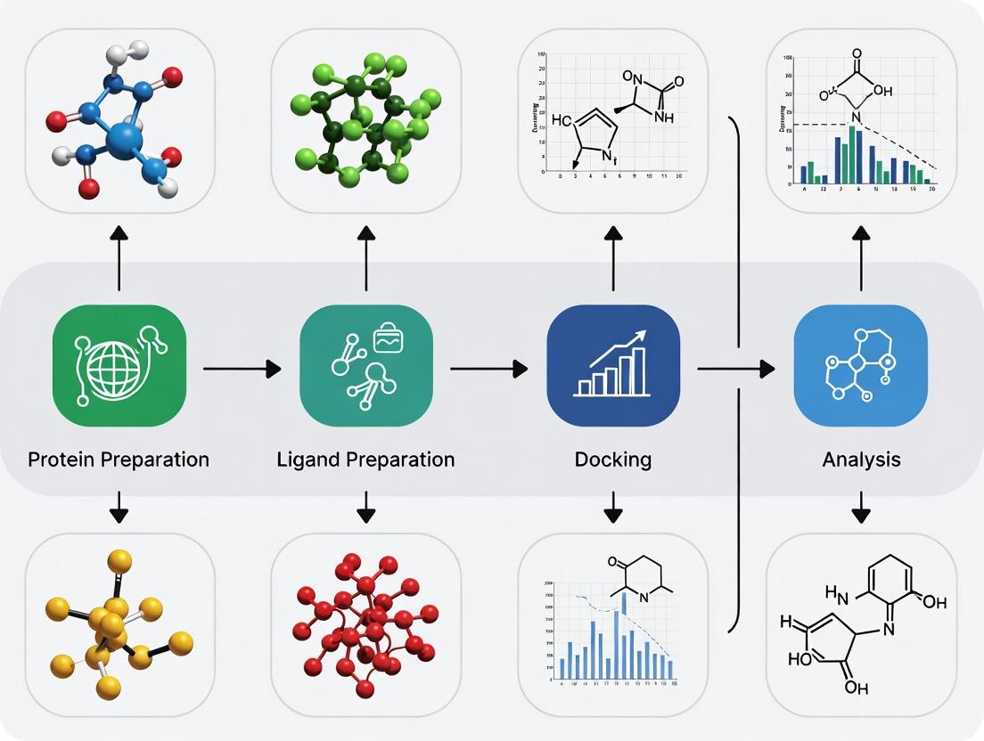
The Integrated Docking Pipeline: A Workflow Diagram
Diagram Title: The Molecular Docking Pipeline Workflow
Key Preparation Steps and Their Impact on Docking Success
Proper file preparation addresses structural imperfections and standardizes inputs. The following table quantifies common issues in raw structural files and the preparation steps that resolve them.
Table 1: Common Issues in Raw Structural Files and Preparation Corrections
| Component | Common Issue in Raw File | Preparation Step | Typical Impact on Docking if Uncorrected |
|---|---|---|---|
| Protein | Missing hydrogen atoms | Protonation at target pH | Severe; incorrect H-bond networks |
| Protein | Missing side chains/loops | Model missing residues | High; false binding site topology |
| Protein | Incorrect protonation states | Assign states (e.g., His, Asp) | High; distorted electrostatic complementarity |
| Protein | Crystallographic waters/ions | Curate (remove/retain) | Moderate to High; false steric clashes |
| Ligand | Incorrect bond orders | Bond order assignment | Severe; incorrect geometry & chemistry |
| Ligand | Missing explicit hydrogens | Protonation (e.g., for pH 7.4) | High; loss of key H-bond interactions |
| Ligand | Poor 3D geometry | Energy minimization | Moderate; increased steric clash penalties |
| Ligand | Multiple tautomers/protomers | Generate relevant states | Moderate; selection of non-bioactive form |
Experimental Protocols for File Preparation
Protocol 1: Standard Protein Preparation from a PDB File
This protocol details the steps to generate a clean, docking-ready protein structure.
- Retrieve & Initial Process: Download the protein structure (e.g., from RCSB PDB). Remove all non-relevant molecules (heteroatoms) except essential cofactors or crystallographic waters in the active site. Remove alternate conformations, keeping the highest occupancy.
- Add Missing Components: Using a modeling suite (e.g., UCSF Chimera, Schrödinger Protein Preparation Wizard), add missing hydrogen atoms. Model any missing loops or side chains using homology or ab initio methods.
- Assign Protonation States: Calculate and assign correct protonation states for amino acid side chains (especially His, Asp, Glu, Lys) at the target pH (typically 7.4). Use empirical pKa calculation tools (e.g., PROPKA).
- Energy Minimization: Perform a restrained energy minimization (RMSD constraint of 0.3 Å on heavy atoms) to relieve steric clashes introduced during hydrogen addition and protonation. This optimizes the hydrogen bonding network.
- Final Output: Export the prepared protein as a clean
.pdbor.pdbqtfile (the latter includes partial charges and atom types for AutoDock-based tools).
Protocol 2: Ligand Preparation from a SMILES String
This protocol converts a 1D chemical identifier into a 3D, energetically optimized docking-ready ligand file.
- Initial Generation: Input the canonical SMILES string into a cheminformatics toolkit (e.g., RDKit, Open Babel) or molecular builder (e.g., Avogadro, Schrödinger LigPrep).
- Generate 3D Conformation: Generate an initial 3D geometry. Ensure correct stereochemistry is defined.
- Optimize Geometry: Perform a conformational search and energy minimization using a molecular mechanics force field (e.g., MMFF94, UFF) to identify a low-energy 3D conformation.
- Assign Charges & States: Calculate and assign appropriate partial atomic charges (e.g., Gasteiger, AM1-BCC). Generate relevant ionization states and tautomers at physiological pH (7.4). Select the most probable protomer or prepare an ensemble.
- Final Output: Export the final, optimized ligand in a docking-compatible format (e.g.,
.mol2,.sdf, or.pdbqt).
The Scientist's Toolkit: Essential Research Reagent Solutions
Table 2: Key Software Tools for Molecular Docking File Preparation
| Tool Name | Category | Primary Function in Preparation | Typical Output Format |
|---|---|---|---|
| UCSF Chimera | Visualization/Modeling | Protein structure repair, H-addition, energy minimization. | .pdb, .mol2 |
| Open Babel | Format Conversion | Converts chemical files between >100 formats, performs basic minimization. | .sdf, .mol2, .pdbqt |
| RDKit | Cheminformatics Library | Programmatic ligand generation, tautomer enumeration, descriptor calculation. | .sdf, .mol2 |
| AutoDock Tools | Docking Suite | Prepares .pdbqt files for AutoDock Vina/GPU, assigns atom types & charges. |
.pdbqt |
| Schrödinger Suite | Commercial Platform | Integrated, robust preparation of proteins (PrepWizard) and ligands (LigPrep). | .mae, .pdb |
| PROPKA | Standalone Algorithm | Predicts pKa values of protein residues to determine protonation states. | Data for manual adjustment |
| PDB2PQR | Web Server/Software | Adds hydrogens, assigns charge & radii, fills missing atoms via force field rules. | .pqr |
Within a thesis focused on preparing protein and ligand files for molecular docking, the initial and most critical step is sourcing a reliable, high-quality protein structure. The choice between an experimentally determined structure from the Protein Data Bank (PDB) and a computationally predicted model from AlphaFold has profound implications for downstream docking accuracy and reliability. This protocol details systematic approaches for sourcing, evaluating, and preparing protein structures for docking studies.
The Protein Data Bank (PDB)
The PDB is the primary repository for experimentally determined 3D structures of proteins, nucleic acids, and complex assemblies. Methods include X-ray crystallography, Nuclear Magnetic Resonance (NMR) spectroscopy, and cryo-Electron Microscopy (cryo-EM).
AlphaFold Database
The AlphaFold Database, hosted by EMBL-EBI, provides access to millions of protein structure predictions generated by DeepMind's AlphaFold2 AI system. It offers near-complete coverage of several proteomes.
Table 1: Quantitative Comparison of PDB and AlphaFold as Structure Sources
| Criterion | Protein Data Bank (PDB) | AlphaFold Database |
|---|---|---|
| Number of Structures | ~220,000 (as of early 2025) | >200 million predictions |
| Resolution (Typical) | High: <2.0 Å (X-ray); Variable (Cryo-EM) | Not applicable (predicted models) |
| Coverage | Limited to experimentally solved structures | Extensive, including proteins with no solved structure |
| Confidence Metric | Experimental resolution, R-factor, clashscore | Per-residue pLDDT score (0-100) |
| Ligand/Co-factor Info | Often includes biologically relevant ligands | Generally excludes ligands and co-factors |
| Conformational State | May represent a specific conformational state | Generally predicts a single, static ground state |
| Update Frequency | New depositions daily | Periodic major releases |
Structure Sourcing and Evaluation Protocol
Protocol 2.1: Decision Workflow for Sourcing a Protein Structure
Objective: To select the most appropriate protein structure source for a given molecular docking project.
Steps:
- Identify Target: Define the protein of interest (UniProt ID preferred).
- Search PDB: Query the PDB (www.rcsb.org) using the UniProt ID or gene name. Filter results by:
- Method: Prioritize X-ray crystallography with resolution ≤ 2.5 Å or Cryo-EM with resolution ≤ 3.5 Å.
- Completeness: Select structures with minimal missing residues in the binding site/region of interest.
- Relevant Ligands: Prefer structures co-crystallized with a substrate, inhibitor, or similar ligand.
- Mutation/Engineered: Avoid structures with mutations unless they are relevant to the study.
- Check for duplicates (same protein under different PDB IDs).
- Evaluate PDB Entry: If a suitable experimental structure exists, proceed to Protocol 2.3.
- Search AlphaFold: If no suitable experimental structure exists, access the AlphaFold Database (alphafold.ebi.ac.uk). Input the UniProt ID.
- Download Structure: Download the predicted model (default is the ranked 0 model, highest confidence).
- Evaluate AlphaFold Model: Proceed to Protocol 2.2 for confidence assessment.
- Final Decision: Apply the decision logic in Diagram 1.
Protocol 2.2: Evaluating an AlphaFold Model for Docking
Objective: To assess the local and global reliability of an AlphaFold-predicted structure for docking.
Materials & Software: AlphaFold model file (.pdb), visualization software (e.g., PyMOL, UCSF ChimeraX), bioinformatics tools.
Steps:
- Analyze Global pLDDT: Open the model. The pLDDT (predicted Local Distance Difference Test) score is typically in the B-factor column. Color the structure by pLDDT (e.g., dark blue >90, light blue 70-90, yellow 50-70, orange <50).
- Interpret pLDDT Scores:
- >90: High accuracy (side-chains reliable).
- 70-90: Confident backbone prediction.
- 50-70: Low confidence; consider the region as potentially disordered.
- <50: Very low confidence; treat as unstructured.
- Focus on Binding Site: Identify the putative binding site (from literature, homology, or server prediction). Examine the pLDDT scores for every residue within 8-10 Å of this site.
- Critical Criterion: For docking, all key binding site residues should have pLDDT > 70.
- Check Predicted Aligned Error (PAE): Analyze the PAE plot (available on the AlphaFold entry page). This estimates positional error between residues. Look for low error (dark blue) within the binding site region, indicating high relative confidence in its geometry.
- Decision: If binding site confidence is high (pLDDT >70, low PAE), the model may be suitable. If confidence is low, consider using a homologous experimental structure from the PDB as a template for comparative modeling.
Protocol 2.3: Evaluating an Experimental PDB Structure
Objective: To assess the quality and suitability of an experimental structure for molecular docking.
Materials & Software: PDB file, validation report from PDB or wwPDB Validation Server, visualization software.
Steps:
- Retrieve Validation Report: On the RCSB PDB entry page, download the validation report PDF or use the wwPDB Validation Server.
- Key Metrics to Examine (Summarize in Table):
- Resolution: The single most important metric. ≤2.0 Å is ideal for docking.
- R-factor / R-free: Measures agreement between the model and experimental data. R-free > 0.30 is concerning.
- Clashscore: Measures steric overlaps. Lower is better (<10 is ideal).
- Ramachandran Outliers: % of residues in disallowed regions. Should be <1-2%.
- Side-Chain Rotamer Outliers: Should be <3%.
- Real Space Correlation (Cryo-EM): Should be >0.8 for the region of interest.
- Visual Inspection in 3D:
- Electron Density/Map: Load the structure with its electron density (2Fo-Fc map for X-ray) or EM map. Verify that the binding site and key side-chains have clear, continuous density.
- Missing Atoms/Residues: Check for gaps in the backbone or missing side-chains (especially in loops near the binding site).
- Alternative Conformations: Note residues with alternate conformations (A, B, etc.); choose the dominant conformation.
- Ligand Occupancy/B-factors: For co-crystallized ligands, ensure high occupancy and reasonable B-factors (not excessively high compared to the protein).
- Decision: Proceed with preparation if the structure passes quality thresholds and the binding site is well-defined.
Table 2: PDB Structure Quality Thresholds for Molecular Docking
| Metric | Ideal Value | Acceptable Value | Action if Unacceptable |
|---|---|---|---|
| Resolution (X-ray) | ≤ 1.8 Å | ≤ 2.5 Å | Seek higher-resolution structure |
| R-free | < 0.25 | < 0.30 | Interpret with extreme caution |
| Clashscore | < 5 | < 10 | May indicate local errors |
| Ramachandran Outliers | < 0.5% | < 2% | Model/refine outlier regions |
| Binding Site Residue Completeness | 100% | >95% (No key residues missing) | Use homology modeling to loop rebuild |
The Scientist's Toolkit: Research Reagent Solutions
Table 3: Essential Tools for Sourcing and Evaluating Protein Structures
| Tool / Resource | Type | Primary Function | Access Link |
|---|---|---|---|
| RCSB Protein Data Bank | Database | Search, visualize, and download experimentally solved structures. | https://www.rcsb.org |
| AlphaFold Database | Database | Search and download AI-predicted protein structures. | https://alphafold.ebi.ac.uk |
| wwPDB Validation Server | Analysis Server | Generate detailed quality reports for any PDB file. | https://validate.rcsb.org |
| PDBsum | Analysis Server | Quick visual summary of PDB structures, including ligands and interactions. | http://www.ebi.ac.uk/pdbsum |
| MolProbity | Software/Server | All-atom structure validation, including clashscore and rotamer analysis. | http://molprobity.biochem.duke.edu |
| PyMOL | Software | Industry-standard visualization and analysis of 3D structures. | https://pymol.org |
| UCSF ChimeraX | Software | Advanced visualization, ideal for cryo-EM maps and AlphaFold models. | https://www.cgl.ucsf.edu/chimerax |
| UniProt | Database | Central hub for protein sequence and functional information (source of UniProt ID). | https://www.uniprot.org |
Visual Workflows and Diagrams
Title: Decision Workflow for Selecting a Protein Structure Source
Title: Guide to Interpreting AlphaFold pLDDT Confidence Scores
For molecular docking, which aims to predict the binding affinity and orientation of a small molecule within a protein's binding site, the quality of the input ligand structure is paramount. Inaccurate ligand representation, particularly concerning stereochemistry and tautomeric state, is a leading cause of docking failure. This document provides application notes and protocols for sourcing, curating, and preparing ligand structures, framed within the essential preprocessing pipeline for reliable docking research.
Major Chemical Databases and Metadata
A critical first step is selecting the appropriate source database. Each repository differs in scope, curation level, and available metadata, impacting ligand suitability for docking.
Table 1: Comparison of Primary Small Molecule Databases
| Database | Primary Scope | Size (Approx.) | Key Metadata for Docking | Stereochemical Integrity | Access |
|---|---|---|---|---|---|
| PubChem | Broad, screening compounds | 110M+ substances | 2D/3D conformers, bioassay data, vendor info. | Variable; often mixture of isomers. | Free |
| ChEMBL | Bioactive, drug-like molecules | 2.4M+ compounds | Target annotation, binding affinity (Ki, IC50), ADMET data. | High, manually curated. | Free |
| PDB Ligand Expo | Experimentally determined in structures | 24,000+ unique ligands | Bound conformation from X-ray/EM, protein context. | High, reflects experimental electron density. | Free |
| ZINC20 | Commercially available for virtual screening | 230M+ purchasable compounds | Vendor catalogs, drug-likeness filters, pre-generated 3D conformers. | Configurations and enantiomers separated. | Free |
| DrugBank | Approved & investigational drugs | 14,000+ drug entries | Detailed pharmacology, mechanisms, targets, pathways. | High, pharmaceutical standard. | Free (core) |
Search Protocol: To identify a target-relevant ligand from ChEMBL:
- Navigate to the ChEMBL web interface or use the
chembl_webresource_clientPython package. - Perform a target search using a standard name (e.g., "EGFR kinase") or UniProt ID.
- From the target page, access the "Browse Compounds" tab.
- Apply filters:
Standard Type= "IC50" or "Ki",Standard Relation= "=",Standard Value≤ 1000 (nM). - Sort by
Standard Valueand select a compound with a reported structure. Export in SDF or MOL2 format.
File Formats and Stereochemical Representation
The chosen file format dictates the amount of structural and chemical information retained.
Table 2: Common Ligand File Formats in Docking
| Format | Extension | 3D Coordinates | Bond Orders | Stereochemistry | Charges | Recommended Use |
|---|---|---|---|---|---|---|
| SDF/MOL | .sdf, .mol | Yes | Explicit | Explicit (chiral centers) | Can be included | Primary exchange format; ideal for database downloads. |
| MOL2 | .mol2 | Yes | Explicit | Explicit | Partial charges (e.g., Gasteiger) | Direct input for many docking suites (e.g., AutoDock). |
| SMILES | .smi, .txt | No (1D) | Implicit | Can be specified (isomeric SMILES) | No | Fast notation; requires 3D conversion for docking. |
| PDB | .pdb | Yes | Implicit (inferred) | Poor (lacks bond order) | No | Avoid for ligands; loss of critical chemistry. |
Protocol: Converting SMILES to 3D with Defined Stereochemistry Objective: Generate a trustworthy 3D conformation from an isomeric SMILES string using RDKit.
Protocol for Ensuring Stereochemical Integrity
This detailed protocol ensures the ligand's 3D structure correctly represents its stereochemical configuration.
Materials & Reagents:
- Software: RDKit, Open Babel, PyMOL/Maestro (for visualization).
- Input: Ligand file (SDF, MOL2) or validated isomeric SMILES.
- Reference: If available, experimental structure (PDB ID of bound ligand).
Procedure:
- Inspection & Validation:
- Load the ligand into a molecular viewer (e.g., PyMOL).
- For tetrahedral chiral centers, verify the correct "handedness" (R vs. S). In PyMOL, use the
show sticks, ligandandutil.cbaycommands for clarity. - For double-bond stereochemistry (E/Z), ensure the correct substituent geometry.
Curation & Correction (if needed):
- If the source file lacks stereochemistry (e.g., a non-isomeric SMILES), consult the primary literature or the database's "Stereochemistry" field to assign it.
- Using RDKit:
Chem.AssignAtomChiralTagsFromStructure(mol)andChem.AssignStereochemistry(mol, cleanIt=True, force=True)can help interpret 3D coordinates into stereochemical tags.
Conformer Generation for Flexible Docking:
- Generate an ensemble of low-energy 3D conformers that respect the fixed chiral centers.
mol = Chem.MolFromMol2File('ligand.mol2') # Generate multiple conformers conformerids = AllChem.EmbedMultipleConfs(mol, numConfs=50, useRandomCoords=True, pruneRmsThresh=0.5, enforceChirality=True) # Optimize each conformer for cid in conformerids: AllChem.MMFFOptimizeMolecule(mol, confId=cid) # Cluster conformers by RMSD and select representatives rmslist = [] for i in range(len(conformerids)): for j in range(i+1, len(conformerids)): rms = AllChem.GetBestRMS(mol, mol, i, j) rmslist.append(rms) # ... (Butina clustering code) ... # Save top 10 diverse conformers writer = Chem.SDWriter('ligandconformers.sdf') for i in selectedconf_ids: writer.write(mol, confId=i) writer.close()- Generate an ensemble of low-energy 3D conformers that respect the fixed chiral centers.
The Ligand Preparation Workflow
Title: Ligand Sourcing and Curation Workflow for Docking
The Scientist's Toolkit: Key Research Reagents & Software
| Item Name | Category | Function in Ligand Preparation |
|---|---|---|
| RDKit | Open-Source Cheminformatics Library | Core toolkit for reading/writing chemical files, stereochemistry handling, 2D->3D conversion, conformer generation, and charge calculation. |
| Open Babel | Chemical File Conversion Tool | Swis-army knife for batch format conversion (e.g., SDF to MOL2) and basic structure optimization. |
| PyMOL / ChimeraX | Molecular Visualization Software | Critical for visual inspection of 3D ligand structures, chiral centers, and alignment to experimental reference. |
| MOE / Schrödinger Maestro | Commercial Suites | Provide integrated, robust pipelines for ligand preparation, including advanced protonation state prediction (Epik) and energy minimization. |
| PDB Ligand Expo | Reference Database | Source of experimentally validated ligand geometries and stereochemistry from Protein Data Bank structures. |
| Gasteiger-Marsili Method | Algorithm | A rapid method for calculating partial atomic charges, often required as input for docking scoring functions. |
| MMFF94/MMFF94s | Force Field | Used for the energy minimization and geometry optimization of generated ligand conformers. |
Molecular docking is a pivotal computational technique in structural biology and drug discovery, used to predict the preferred orientation and binding affinity of a small molecule (ligand) to a target macromolecule (receptor). The selection and definition of the binding site critically influence the accuracy and efficiency of docking simulations. This protocol details the progression from using known active site coordinates to employing blind docking strategies, framed within the essential preparatory steps for protein and ligand file preparation.
The choice of docking strategy is dictated by the availability of structural information on the target protein.
Table 1: Comparative Analysis of Docking Site Definition Strategies
| Strategy | Description | Typical Grid Box Dimensions (ų) | Computational Cost | Use Case |
|---|---|---|---|---|
| Known Coordinates (Site-Specific) | Docking directly into a well-characterized active site, often from a co-crystallized ligand. | 20x20x20 - 25x25x25 | Low | High-confidence active site; lead optimization. |
| Literature/Sequence-Based | Defining the site based on known catalytic residues or homologous structures. | 22x22x22 - 30x30x30 | Low-Medium | Known functional site but no ligand-bound structure. |
| Pocket Detection | Using algorithms (e.g., FPocket, SiteMap) to identify potential binding cavities. | Varies per detected pocket (~25³ per pocket) | Medium | Novel targets or allosteric site discovery. |
| Blind Docking | Scanning the entire protein surface for potential binding sites. | Entire protein surface (e.g., 60x60x60) | Very High | Unknown binding site or fragment-based screening. |
Experimental Protocols
Protocol 2.1: Preparation of Protein and Ligand Files
This is a foundational step for all subsequent docking strategies.
A. Protein Preparation:
- Source & Clean: Obtain a 3D structure (.pdb) from the PDB database. Remove all non-protein atoms (water, ions, previous ligands) except crucial co-factors.
- Add Hydrogens & Charges: Use tools like UCSF Chimera, AutoDockTools, or Schrödinger's Protein Preparation Wizard. Protonate residues at physiological pH (e.g., 7.4). Assign partial atomic charges (e.g., Gasteiger charges).
- Optimize Structure: Minimize the protein's energy, particularly fixing steric clashes in side chains, while typically keeping the backbone fixed.
- Output Format: Save the prepared protein in the required format (e.g., .pdbqt for AutoDock Vina/GPU, .mae for Schrödinger).
B. Ligand Preparation:
- Source: Draw or obtain ligand structure (.sdf, .mol2) from databases like PubChem or ZINC.
- Optimize Geometry: Perform energy minimization using molecular mechanics (e.g., MMFF94).
- Generate Tautomers/States: At pH 7.4, generate possible ionization states and tautomers.
- Assign Charges: Assign appropriate partial charges compatible with the docking software.
- Set Rotatable Bonds: Identify and define rotatable bonds for flexible docking. For rigid docking, treat the ligand as rigid.
Protocol 2.2: Site-Specific Docking with Known Coordinates
- Software: AutoDock Vina, AutoDock GPU, Glide (SP/XP).
- Steps:
- Identify the 3D coordinates (X, Y, Z) of the known binding site centroid from the co-crystallized ligand or catalytic residues.
- Define a grid box centered on these coordinates. The size should be large enough to accommodate ligand movement (see Table 1).
- Configure the docking software with the prepared protein (.pdbqt) and ligand(s) (.pdbqt), specifying the grid box coordinates and size.
- Run the docking simulation. For Vina, set
num_modesto 10 andexhaustivenessto 8-32. - Cluster results by RMSD and analyze top-ranked poses by binding affinity (ΔG in kcal/mol).
Protocol 2.3: Blind Docking Protocol
- Software: AutoDock Vina/GPU with large grid, CB-Dock2, SwissDock.
- Steps:
- Prepare the protein and ligand as in Protocol 2.1.
- Define the Global Search Space: Set the grid box to encompass the entire protein or a major portion of it. For a typical protein, dimensions of 60x60x60 ų or larger may be needed. Ensure the grid center covers the protein's geometric center.
- Increase Search Exhaustiveness: To adequately sample the vast search space, significantly increase the search parameter (e.g.,
exhaustivenessin Vina to 32-128). - Execute the docking run. This is computationally intensive and benefits from GPU acceleration.
- Post-process all output poses. Use cluster analysis to identify consensus binding regions. Evaluate the top clusters not only by score but also by complementarity (e.g., via visualization in PyMOL/Chimera).
Visualization of Workflows
Title: Decision Workflow for Docking Strategy Selection
Title: Ligand Preparation Protocol Steps
The Scientist's Toolkit: Research Reagent Solutions
Table 2: Essential Software & Resources for Docking Preparation
| Item | Category | Function/Brief Explanation |
|---|---|---|
| UCSF Chimera | Visualization/Preparation | Opensource tool for interactive visualization, basic cleanup, adding hydrogens, and energy minimization of protein structures. |
| AutoDockTools (ADT) | Preparation | GUI for preparing .pdbqt files, setting up grid boxes, and defining rotatable bonds for AutoDock suite. |
| Open Babel / RDKit | Ligand Preparation | Toolkits for converting chemical file formats, energy minimization, and generating ligand conformers. |
| Schrödinger Suite | Commercial Platform | Integrated platform (Maestro GUI) offering robust, automated protein & ligand prep (Protein Prep Wizard, LigPrep), and multiple docking engines (Glide). |
| PyMOL | Visualization | Industry-standard for high-quality rendering and analysis of docking results and protein-ligand interactions. |
| PDB Database (rcsb.org) | Data Repository | Primary source for experimentally-determined 3D structures of proteins and nucleic acids. |
| PubChem / ZINC | Ligand Database | Vast public repositories of small molecule structures and commercially available compounds for virtual screening. |
| FPocket | Pocket Detection | Open-source tool for detecting and analyzing potential binding pockets on protein surfaces. |
| GNINA / AutoDock GPU | Docking Engine | High-performance, open-source docking software utilizing CNN scoring or GPU acceleration for fast simulations. |
| CB-Dock2 | Web Server | User-friendly web server for automated blind docking, integrating cavity detection and Vina docking. |
Hands-On Preparation: A Step-by-Step Workflow for Protein and Ligand Files
In the broader thesis of preparing files for molecular docking, this initial step is critical. The quality and appropriateness of the protein structure directly determine the reliability of subsequent docking simulations and virtual screening campaigns. An uncleaned Protein Data Bank (PDB) file, containing extraneous components like crystallographic water molecules, non-essential ions, co-factors, and redundant alternate conformations, can lead to false-positive binding sites, steric clashes, inaccurate energy calculations, and ultimately, failed experiments. This protocol details the systematic isolation of the target protein chain and the removal of non-essential elements to create a "cleaned" receptor file, establishing a robust foundation for subsequent steps like protonation, energy minimization, and binding site definition.
Key Considerations and Quantitative Data
The decision to retain or remove components depends on the biological context of the docking study. The following table summarizes common PDB file components and the rationale for their treatment.
Table 1: Treatment Guidelines for Common PDB Components in Preliminary Cleaning
| PDB Component | Typical Removal? | Rationale & Exceptions | Recommended Tool Action |
|---|---|---|---|
| Water Molecules | Usually, but context-dependent | Remove all. Retain only catalytic waters or those in deeply buried, structurally critical pockets. | Bulk deletion with selective manual inspection. |
| Non-essential Ions (Na+, Cl-) | Yes | Typically crystallization artifacts. Remove unless integral to protein structure/function. | Remove by heteroatom/chain ID. |
| Essential Divalent Ions (Mg2+, Zn2+, Ca2+) | No | Often catalytic or structural. Retain and ensure proper charge/parameterization later. | Identify and preserve. |
| Small Molecule Co-factors (NAD, HEM, ATP) | Context-dependent | Remove if not involved in target binding site. Retain if part of the active site or if docking involves this site. | Remove by HETATM code; retain if functionally crucial. |
| Alternate Conformations | Yes | Represent crystallographic uncertainty. Retain only the highest occupancy or most biologically relevant conformer. | Choose single conformer (usually Atom 'A' of group). |
| Unnecessary Protein Chains | Yes | Remove symmetry mates, fusion proteins, or irrelevant chains from complexes. Isolate the biologically relevant monomer or oligomer. | Select by chain ID. |
| Ligands from Co-crystal Structures | Usually | Remove the native ligand to prepare the apo structure for new ligand docking, unless studying competitive binding. | Delete by HETATM/residue name. |
Detailed Experimental Protocols
Protocol 1: Manual Cleaning Using UCSF ChimeraX
This protocol offers fine-grained control for a single or few structures.
Materials & Reagents:
- Software: UCSF ChimeraX (Current version: 1.8).
- Input File: Target PDB file (e.g.,
7XYZ.pdb). - Computing Environment: Standard desktop workstation.
Methodology:
- Open and Inspect:
- Launch ChimeraX. Open your structure:
open 7XYZ.pdb. - Use the
summarycommand to list all chains, ligands, and residues. - Visually inspect the structure (
Viewer) to identify the binding site, co-factors, and water networks.
- Launch ChimeraX. Open your structure:
Remove Water Molecules:
- In the Command Line, execute:
remove solvent - To inspect and selectively delete specific waters, select them manually (click) and press
Delete.
- In the Command Line, execute:
Remove Unnecessary Chains:
- Identify the target chain (e.g., Chain A). Select all atoms not in Chain A:
select ~:Atheninvert - Delete the selection:
delete sel
- Identify the target chain (e.g., Chain A). Select all atoms not in Chain A:
Handle Heteroatoms (HETATM):
- List all hetero residues:
info hetero - To remove a specific co-factor (e.g., SO4):
remove resname SO4 - To retain a crucial co-factor (e.g., HEM), take no action.
- List all hetero residues:
Process Alternate Locations:
- Use the
Model Panel(Favorites → Model Panel). Under the "Altlocs" tab, for each residue, choose the conformer with the highest occupancy (e.g., "A") and delete others.
- Use the
Save the Cleaned Structure:
- Save the processed model:
save clean_7XYZ.pdb
- Save the processed model:
Protocol 2: Automated/Batch Cleaning Using BioPython PDBParser
This protocol is suitable for processing multiple structures programmatically.
Materials & Reagents:
- Software: Python 3.9+ with BioPython, pandas libraries.
- Input Files: Directory containing multiple PDB files.
- Computing Environment: Any Python-capable system.
Methodology:
Visualizations
Workflow Diagram for Protein Cleaning
Diagram Title: Decision Workflow for Preliminary Protein Structure Cleaning
The Scientist's Toolkit: Research Reagent Solutions
Table 2: Essential Software Tools for Protein Structure Cleaning
| Tool Name | Primary Function | Use Case in This Step | Key Feature for Cleaning |
|---|---|---|---|
| UCSF ChimeraX | Interactive visualization & analysis | Manual inspection and selective deletion. | Intuitive GUI, command line, remove solvent, select by attributes. |
| PyMOL | Molecular visualization system | Manual cleaning and high-quality rendering. | Powerful selection algebra (sele chain A and not resn HOH). |
| BioPython PDB | Python library for structural bioinformatics | Automated, batch processing of many PDB files. | Programmatic parsing and editing of PDB files. |
| PDBrenum | Web server/tool for PDB renumbering | Standardizing residue numbering post-cleaning. | Ensures consistent numbering for downstream steps. |
| MolSoft ICM Browser | Free web-based 3D molecule viewer | Quick initial inspection before detailed cleaning. | No installation required, rapid online viewing. |
Within the broader thesis on preparing files for molecular docking, this step is critical. Protein structures from sources like the Protein Data Bank (PDB) are often incomplete or lack essential physicochemical details. This stage ensures the protein model is biochemically realistic, with correct protonation states, filled structural gaps, and proper formal charges, forming a reliable foundation for docking simulations.
The table below summarizes the core tasks, common issues, and primary software solutions used for protein structure completion and optimization.
Table 1: Overview of Protein Structure Completion and Optimization Tasks
| Task | Common Issue in Raw PDB | Critical Parameters | Primary Tools/Software |
|---|---|---|---|
| Hydrogen Addition | Hydrogens are rarely resolved in X-ray structures. | Protonation state at given pH, tautomer selection. | H++ (web), PDB2PQR, MOE, ChimeraX. |
| Missing Side Chains | Electron density for terminal residues or long side chains (e.g., Lys, Arg) may be missing. | Rotamer library quality, steric clash avoidance. | SCWRL4, MODELLER, PDBFixer, Rosetta. |
| Missing Loops/Residues | Disordered regions lacking coordinates. | Loop modeling algorithm, template selection. | MODELLER (homology), Rosetta de novo, Swiss-Model. |
| Charge Assignment | Formal and partial charges are not standardized in PDB. | Force field compatibility (e.g., AMBER, CHARMM). | PDB2PQR, Antechamber (AMBER), MOE, GROMACS pdb2gmx. |
| Disulfide Bond Detection | Cysteine bridges may be annotated incorrectly or not at all. | Cysteine S–S distance (~2.0–2.1 Å). | ChimeraX, Coot, PyMOL. |
Experimental Protocols
Protocol 1: Comprehensive Preparation Using UCSF ChimeraX This protocol provides a graphical user interface (GUI)-based workflow suitable for most standard preparations.
- Load Structure: File → Open, select your PDB file.
- Add Hydrogens: Tools → Structure Editing → Add Hydrogens. Specify the correct pH (typically 7.4) for protonation state prediction.
- Add Missing Atoms: Tools → Structure Editing → Dunbrack Rotamer Library. Use “Add” to fill missing side chains. For missing loops, use Tools → Structure Editing → Model Loops (requires sequence alignment).
- Assign Charges: Tools → Structure Editing → Add Charge. Select the appropriate force field (e.g., AMBERff14SB for standard proteins).
- Energy Minimization: To resolve steric clashes introduced during addition. Tools → Structure Editing → Minimize Structure (NAMD or AMBER interface).
- Validation: Use Tools → Structure Analysis → Validate (MolProbity) to check for clashes, Ramachandran outliers, and rotamer issues.
Protocol 2: Automated, Scriptable Preparation Using PDB2PQR & APBS This protocol is ideal for batch processing and ensuring proper charge assignment for subsequent electrostatic calculations.
- Input Preparation: Ensure your PDB file has the target protein chain(s) of interest.
- Run PDB2PQR: Execute via command line or web server.
- Handle Missing Residues: PDB2PQR will warn of missing atoms. For large gaps, pre-fill using a tool like MODELLER or PDBFixer before running PDB2PQR.
- Output: The
.pqrfile contains added hydrogens, assigned partial charges, and atomic radii. The accompanying.infile is ready for electrostatic potential calculation with APBS.
Protocol 3: Homology Modeling for Missing Loops/Residues Using MODELLER This protocol is for significant missing segments (>5 residues).
- Sequence & Alignment: Extract the target protein sequence from the PDB. Identify missing residue ranges. Perform a sequence search (e.g., BLAST) against the PDB to find a homologous template containing the missing region.
- Prepare Alignment File: Create a sequence alignment file (PIR format) between target and template, marking the missing residues as gaps in the target structure.
- Write MODELLER Script: Create a Python script (
model_loop.py) that:- Loads the incomplete PDB structure.
- Reads the alignment.
- Restricts modeling to the selected loop region to minimize disturbance to the known structure.
- Generates multiple models (e.g., 100).
- Select Best Model: Run the script, then select the model with the lowest MODELLER objective function and favorable DOPE assessment score. Visually inspect the loop geometry.
Visualization of Workflows
Title: Protein Structure Optimization Workflow
The Scientist's Toolkit: Research Reagent Solutions
Table 2: Essential Software Tools for Structure Completion
| Tool/Solution | Primary Function | Key Feature for Docking Prep |
|---|---|---|
| UCSF ChimeraX | Integrated molecular visualization and modeling. | GUI-based comprehensive tool for adding H+, charges, fixing side chains, and loop modeling via plugins. |
| PDB2PQR Server | Automated pipeline for adding hydrogens, missing atoms, and assigning charges. | Integrates PropKa/pKa for pH-based protonation, outputs files compatible with APBS and major docking suites. |
| SWISS-MODEL | Automated protein structure homology modeling. | Reliable server for modeling large missing regions if a suitable template exists. |
| MODELLER | Homology modeling of structures and loops. | Programmatic control for modeling specific missing loops within an existing framework. |
| AMBER Tools (Antechamber) | Parameterization of molecules and charge assignment. | Essential for assigning GAFF force field parameters and RESP charges to non-standard ligands or residues. |
| MolProbity (via Phenix/ChimeraX) | Structure validation suite. | Checks steric clashes, rotamer outliers, and Ramachandran plot quality post-optimization. |
| Rosetta (RosettaCM, Relax) | High-resolution structure prediction and design. | Powerful de novo loop modeling when no homologous template is available. |
This protocol details the critical step of ligand preparation within a molecular docking pipeline. The 3D structure of a small molecule, as obtained from databases, is often incomplete or unrefined. Incorrect bond order, unspecified stereochemistry, non-representative tautomeric forms, and improper protonation states are major sources of docking failures. This stage ensures the ligand's electronic and structural representation is chemically accurate and physiologically relevant at the target protein's environmental pH, thereby increasing the reliability of subsequent docking poses and scoring.
Table 1: Impact of Ligand Optimization on Docking Outcomes
| Optimization Parameter | Docking Success Rate (Unoptimized) | Docking Success Rate (Optimized) | Typical Software/Tool Used |
|---|---|---|---|
| Correct Bond Order Assignment | ~40-50% | >85% | RDKit, Open Babel, LigPrep (Schrödinger) |
| Tautomer Enumeration/Sampling | Varies by compound class | Improves pose RMSD by up to 2.0 Å | Epik, MOE, ChemAxon Calculator |
| Protonation at pH 7.4 ± 0.5 | ~60% | >90% (for relevant targets) | LigPrep, Epik, Open Babel (--addpH), Moka |
| Formal Charge Assignment | ~70% | ~98% | Open Babel, MarvinSuite, ChemAxon |
Table 2: Recommended Parameters for Protonation State Prediction
| Software | Default pKa Model | Target pH Range | Recommended for |
|---|---|---|---|
| Schrödinger Epik | Empirical, quantum-mechanical | 0.0 - 14.0 | High-accuracy, drug-like molecules |
| ChemAxon Marvin | Microspecies distribution | User-defined | Rapid batch processing |
| Open Babel | Empirical rules-based | User-defined | Open-source workflows, standard molecules |
| MOE (Chemical Computing Group) | Stochastic titration | 5.0 - 9.0 | Integrated structure-based design |
Experimental Protocol: Comprehensive Ligand Preparation
Protocol 3.1: Standardized Ligand Preparation Workflow Using Open-Source Tools
Objective: To generate a 3D, energetically minimized, and pH-corrected ligand structure from a 2D SDF or SMILES string.
Materials & Reagents:
- Input File: Ligand structure in SDF, MOL2, or SMILES format.
- Software: Open Babel (v3.1.1+), RDKit (2023.09+), UCSF Chimera (or PyMOL for visualization).
- System: Linux/macOS/Windows command line or Python scripting environment.
Procedure:
- Structure Standardization and Sanitization (RDKit):
Bond Order and Formal Charge Assignment (Open Babel):
Protonation State Generation at Target pH (Open Babel):
Tautomer Enumeration (RDKit - Basic):
Energy Minimization (RDKit/Open Babel):
Protocol 3.2: High-Fidelity Preparation Using Schrödinger Suite
Objective: To perform exhaustive ligand state sampling using industry-standard, physics-based models.
Materials & Reagents:
- Software: Schrödinger Suite (Maestro, LigPrep, Epik).
- Input: SMILES or 2D/3D structure file.
- System: Linux server with Schrödinger installation.
Procedure:
- LigPrep Execution: Run the
ligpreputility.
- Output Analysis: The output SDF contains multiple ligand states, each with a relative energy penalty and predicted probability at the target pH. Select the lowest penalty state for standard docking, or use an ensemble for more comprehensive screening.
Visual Workflows
Diagram 1: Ligand Optimization Workflow for Docking
Diagram 2: Decision Logic for Ligand State Selection
The Scientist's Toolkit: Research Reagent Solutions
Table 3: Essential Software Tools for Ligand Optimization
| Tool Name | Type/Category | Primary Function in Optimization | Key Feature |
|---|---|---|---|
| RDKit | Open-source Cheminformatics Library | Bond order perception, sanitization, basic tautomer enumeration, 3D generation. | Programmable via Python, robust and free. |
| Open Babel | Open-source Chemical Toolbox | File format conversion, 3D coordinate generation, rule-based protonation, minimization. | Command-line friendly, supports batch processing. |
| Schrödinger LigPrep/Epik | Commercial Suite Module | High-accuracy pKa prediction, tautomer generation, desaltation, stereoisomer generation. | Physics-based models, integrated with Maestro GUI. |
| ChemAxon MarvinSuite | Commercial Cheminformatics Suite | pKa and tautomer prediction, chemical structure drawing and standardization. | Excellent for batch processing and microspecies analysis. |
| Moka (Molecular Discovery) | Commercial Tool | Specifically for protonation state prediction and free energy perturbation. | Focused on accurate protonation for binding sites. |
| UCSF Chimera | Visualization & Modeling | Interactive protonation (AddH), structure cleanup, basic energy minimization. | User-friendly GUI, ideal for manual inspection and correction. |
Within the workflow of preparing files for molecular docking research, file format conversion is a critical, non-negotiable step. Molecular docking software suites, such as AutoDock Vina, AutoDock4, DOCK6, and Schrödinger's Glide, require inputs in specific, often proprietary, formats that contain essential molecular information not present in standard PDB or SDF files. This step involves adding partial atomic charges, defining rotatable bonds (for ligands), merging non-polar hydrogens, and assigning atom types specific to the force field of the docking program. Failure to execute this conversion correctly leads to docking failures or physically meaningless results, undermining all subsequent analyses.
Common File Formats in Molecular Docking
The following table summarizes the primary file formats encountered, their typical contents, and the major docking tools that utilize them.
Table 1: Key File Formats for Molecular Docking
| Format | Primary Use | Key Features/Contents | Common Docking Tools |
|---|---|---|---|
| PDB | Initial input for proteins/ligands. | Atomic coordinates, atom/residue names, chain identifiers. Universal starting point. | None (requires conversion). |
| SDF/MOL2 | Initial input for small molecules. | 3D coordinates, bond connectivity, partial charges (sometimes). | Requires conversion for most tools. |
| PDBQT (AutoDock) | Docking input for receptor and ligand. | Adds partial charges (q), atom types (t), and rotatable bond records (TORSDOF). Merges non-polar hydrogens. |
AutoDock Vina, AutoDock4, SMINA. |
| MOL2 (Sybyl) | Docking input for ligand and sometimes receptor. | Detailed bond and atom type definitions, partial charges, substructure records. | DOCK6, Lead Finder, MOE. |
| PDB2 | Internal format for GOLD. | Similar to PDB but with specific syntax for flexibility. | GOLD Suite. |
| MAE (Macromodel) | Internal format for Schrödinger. | Contains extensive force field parameters and properties. | Glide, Desmond. |
Core Conversion Protocols
Protocol: Generating PDBQT Files for AutoDock Vina/AutoDock4
This protocol uses the open-source tools AutoDockTools (ADT) and Open Babel.
A. Ligand Preparation (Using Open Babel Command Line):
- Input: A ligand file in SDF or MOL2 format (
ligand.sdf). - Add Hydrogens and Charges: Ensure the ligand has appropriate protonation states and partial charges. For Vina, Gasteiger charges are commonly used.
- Manual Checking/Editing (Optional but Recommended): Load the
ligand_h.pdbqtfile into ADT to visually verify and define rotatable bonds. The root of the ligand is automatically assigned but can be manually adjusted.
B. Protein/Receptor Preparation (Using AutoDockTools - GUI Method):
- Input: A cleaned protein PDB file (from Step 3: Cleaning and Optimization).
- Load Molecule: In ADT, use
File > Read Moleculeto open your protein PDB file. - Edit Hydrogens: Use
Edit > Hydrogens > Addto add all polar hydrogens. Then,Edit > Hydrogens > Removeto select "Remove Non-Polar." - Add Charges: Select
Edit > Charges > Add Kollman Charges. - Assign AD4 Types: Choose
Edit > Atoms > Assign AD4 Type. - Save as PDBQT: Finally, select
Grid > Macromolecule > Chooseand save the resulting PDBQT file.
Protocol: Generating MOL2 Files with Partial Charges for DOCK6
A. Using UCSF Chimera:
- Input: A ligand SDF or a receptor PDB file.
- Add Charges: For ligands, use
Tools > Structure Editing > Add Charge. Select the AM1-BCC method (recommended for organic molecules in DOCK6). For receptors, useTools > Structure Editing > Add Chargeand select the AMBER ff14SB force field. - Save File: Use
File > Save Molecule As...and select "Sybyl Mol2" as the format. Ensure the option to save charges is selected.
B. Using antechamber/ACPYPE for Ligands (Automated, High-Quality):
- Input: Ligand in MOL2 or PDB format (
LIG.mol2). - Determine Charge: Calculate the net charge of your ligand at physiological pH (e.g., +1, 0, -1).
- Run antechamber & acpype: This pipeline generates GAFF force field parameters and a correctly formatted MOL2.
- Output: The final MOL2 file for docking is typically named
LIG_gaff.acpype/LIG_gaff_NEW.mol2.
Workflow and Decision Pathway
Diagram Title: File Format Conversion Decision Workflow
The Scientist's Toolkit: Essential Reagents & Software
Table 2: Essential Tools for File Format Conversion
| Tool / Reagent | Category | Primary Function | Key Consideration |
|---|---|---|---|
| AutoDockTools (ADT/MGLTools) | GUI Software | Prepares PDBQT files for AutoDock suite. Visual definition of rotatable bonds and docking box. | Python 2.7-based; legacy but essential for Vina prep. |
| Open Babel | Command-Line & Library | Universal chemical format converter. Can add hydrogens, charges, and generate PDBQT. | Fast and scriptable; charge models are simpler than quantum methods. |
| UCSF Chimera | GUI Software | High-quality structure visualization and editing. Excellent for adding charges (AM1-BCC, AMBER) and saving MOL2. | User-friendly; integrates well with computational workflows. |
| antechamber/ACPYPE | Command-Line Tool | Generates high-quality force field parameters (GAFF) and MOL2 files with AM1-BCC charges for ligands. | Industry standard for ligand parameterization; requires net charge input. |
| Schrödinger Maestro/Protein Prep Wizard | Commercial Suite | Integrated environment for preparing MAE files for Glide docking. Handles protein refinement, H-bond assignment, and restrained minimization. | Comprehensive but license-dependent. |
| GOLD Suite (Hermes) | Commercial Suite | Prepares ligands and proteins in the native PDB2 format for GOLD docking. Handles binding site definition and flexibility. | License-dependent; specific to the GOLD algorithm. |
| RDKit | Programming Library | Python/C++ library for cheminformatics. Can be scripted for custom conversion pipelines and charge calculations. | Highly flexible for advanced users and automated workflows. |
| AMBER/GAFF Force Field | Parameter Set | Provides the physical models for atomic partial charges and van der Waals parameters used in high-quality MOL2 file creation. | The antechamber tool applies GAFF parameters. |
This application note details a critical workflow in computational drug discovery: preparing a target protein and a compound library for virtual screening (VS). This process is a foundational step in the broader thesis of "Optimization of File Preparation Protocols for Robust and Reproducible Molecular Docking Research." Accurate preparation of both protein and ligand structures is paramount to the success of downstream docking simulations, directly impacting hit identification rates and the validity of structure-based drug design campaigns.
Protein Preparation: Angiotensin-Converting Enzyme (ACE, PDB ID: 1O86)
Initial Acquisition and Assessment
The crystal structure of human testicular angiotensin-converting enzyme (tACE) in complex with the inhibitor lisinopril was retrieved from the Protein Data Bank (PDB ID: 1O86). Key initial parameters are summarized in Table 1.
Table 1: Initial Assessment of PDB Entry 1O86
| Parameter | Value / Observation |
|---|---|
| Resolution | 2.0 Å |
| Chains | A (Catalytic Domain), B (C-terminal domain) |
| Relevant Ligand | Lisinopril (bound to Chain A) |
| Missing Residues | Minor loops in non-catalytic regions |
| Water Molecules | 296 crystallographic waters |
| Original Publication | Natesh et al., Biochemistry 2003 |
Detailed Protein Preparation Protocol
This protocol utilizes standard software suites (e.g., UCSF Chimera, Schrödinger Maestro's Protein Preparation Wizard, or similar).
Structure Loading and Initial Cleaning:
- Load the PDB file into the preparation software.
- Remove Unnecessary Components: Delete all water molecules, ions, and buffer molecules initially. The co-crystallized ligand (lisinopril) should be retained for reference during binding site definition.
- Chain Selection: For virtual screening focused on the canonical zinc-binding site, retain only Chain A. Chain B can be removed to simplify the system.
Missing Component Modeling:
- Identify and model any missing side chains or short loops using standard rotamer libraries and loop modeling algorithms within the software. For 1O86, this is minimal.
Hydrogen Addition and Protonation States:
- Add all hydrogen atoms to the protein structure.
- Critical Step: Optimize the protonation states of histidine, aspartic acid, glutamic acid, lysine, and arginine residues at the target pH (typically pH 7.4 for physiological conditions).
- Pay Special Attention to the Catalytic Site: The zinc-coordinating residues (His383, His387, Glu411) must be correctly protonated. The two histidines should be in the neutral (HD1 or HE2 protonated) state to coordinate Zn²⁺.
Structure Optimization and Minimization:
- Perform a constrained energy minimization (e.g., using the OPLS4 or CHARMm force field) to relieve steric clashes introduced by hydrogen addition and side-chain adjustments. The protein backbone is typically restrained to its original crystallographic conformation to maintain the validated binding site geometry.
Binding Site Definition:
- Define the docking grid or search space. Using the coordinates of the bound lisinopril as a center, generate a grid box of sufficient size (e.g., 20 Å x 20 Å x 20 Å) to encompass the active site pocket and adjacent sub-pockets.
Workflow: Protein Structure Preparation
Ligand Library Preparation
Library Curation
A diverse library of 10,000 small molecules was sourced from the ZINC15 database. Selection criteria are outlined in Table 2.
Table 2: Ligand Library Curation Criteria
| Criterion | Value / Filter | Rationale |
|---|---|---|
| Source | ZINC15 'Lead-Like' subset | Focus on drug-like starting points |
| Molecular Weight | 250 - 350 Da | Adherence to lead-like properties |
| LogP | -2.0 to 4.0 | Optimal for solubility and permeability |
| Rotatable Bonds | ≤ 7 | Favorable for oral bioavailability |
| Formal Charge | -2 to +2 at pH 7.4 | Physiological relevance |
| Structural Diversity | Tanimoto coefficient < 0.8 (FP2) | Maximize chemical space coverage |
Detailed Ligand Preparation Protocol
Protocol based on tools like Open Babel, RDKit, or Schrödinger LigPrep.
Format Standardization and Cleaning:
- Convert all library compounds from their source format (e.g., SDF) into a consistent working format (e.g., MAE, MOL2).
- Remove counterions, salts, and solvents.
- Check for and correct invalid valences or unusual atom types.
Tautomer and Stereoisomer Generation:
- For each input molecule, generate relevant tautomeric forms and stereoisomers (specifying up to a maximum, e.g., 32 per ligand) likely to exist at physiological pH.
Energy Minimization and 3D Optimization:
- Generate a low-energy 3D conformation for each ligand variant using a molecular mechanics force field (e.g., MMFF94s). This provides a reasonable starting geometry for flexible docking.
Assignment of Partial Charges and Protonation States:
- Calculate Gasteiger or similar partial atomic charges.
- Critical Step: Assign the correct protonation state (major microspecies) at pH 7.4 ± 2.0 using an algorithm like Epik. This ensures ligands are prepared in a physiologically relevant form.
Final Format Export:
- Export the final, prepared library of 3D structures in a docking-ready format compatible with the chosen docking software (e.g., SDF, MOL2, or specific vendor format).
Workflow: Ligand Library Preparation
The Scientist's Toolkit: Research Reagent Solutions
Table 3: Essential Materials and Tools for Preparation
| Item / Software | Category | Primary Function in Preparation |
|---|---|---|
| RCSB Protein Data Bank (PDB) | Database | Source of high-resolution 3D protein structures (e.g., 1O86). |
| UCSF Chimera / ChimeraX | Visualization & Prep | Open-source tool for initial structure inspection, cleaning, and basic hydrogen addition. |
| Schrödinger Maestro Suite | Commercial Software | Integrated platform for comprehensive protein (Protein Prep Wizard) and ligand (LigPrep) preparation, including advanced protonation state sampling. |
| Open Babel / RDKit | Open-Chem Informatics | Toolkits for command-line or scripted batch conversion, filtering, and basic preparation of ligand libraries. |
| ZINC15 / ChEMBL | Compound Database | Repositories of commercially available or bioactive small molecules for library building. |
| MOE (Molecular Operating Environment) | Commercial Software | Alternative suite offering robust protein modeling and ligand preparation workflows. |
| AutoDock Tools / MGLTools | Free Docking Prep | Utilities specifically for preparing files for the AutoDock/Vina docking engines. |
| Force Fields (OPLS4, CHARMm) | Parameter Set | Sets of mathematical functions and constants used during energy minimization to model molecular geometry and energetics. |
Beyond the Basics: Solving Common Problems and Optimizing for Accuracy
Within the broader thesis on preparing files for molecular docking research, robust protocols for identifying and correcting common structural file errors are foundational. These errors, if unaddressed, lead to failed simulations, inaccurate results, and irreproducible science.
Errors typically arise during file format conversion, topology assignment, and parameterization. The table below quantifies the frequency of common errors identified in a recent survey of pre-processing tools.
Table 1: Prevalence and Impact of Common File Preparation Errors
| Error Type | Reported Frequency (%) | Primary Cause | Typical Consequence |
|---|---|---|---|
| Parsing/Syntax Error | 45 | Improper formatting, missing columns, non-standard delimiters | Immediate failure of simulation or docking run |
| Missing Hydrogen Atoms | 38 | Extraction from X-ray structures (no H atoms resolved) | Incorrect protonation, hydrogen bonding, and charge |
| Missing Heavy Atoms | 12 | Broken residues in PDB files, ligand extraction errors | Severe structural gaps and force field assignment failures |
| Force Field Incompatibility | 85 | Lack of parameters for novel ligands/moieties | Simulation crash or inaccurate molecular mechanics |
Experimental Protocols for Troubleshooting
Protocol 1: Systematic Diagnosis of Parsing and Atomistic Errors Objective: To identify and rectify syntax errors and missing atoms in protein-ligand structure files.
- Visual Inspection: Load the initial structure file (e.g., PDB) in a molecular viewer (e.g., PyMOL, UCSF Chimera). Visually scan for chain breaks, unusual bond lengths, and grossly missing fragments.
- Formal Validation: Run the file through the PDB validation server (for PDB files) or the
pdbfixerutility. This will formally report on missing atoms, residues, and steric clashes. - Tool-Based Repair: For missing heavy atoms in proteins, use
pdbfixerto add missing residues and atoms. For missing hydrogens and protonation states, usereduceor thepdb4ambersuite. - Ligand-Specific Checking: For ligands, use the
Grade2web server orantechamberto ensure chemical validity and generate correct connectivity.
Protocol 2: Resolving Force Field Incompatibilities for Novel Ligands Objective: To generate missing force field parameters for small molecule ligands not in standard libraries.
- Ligand Preparation: Start with a validated, 3D ligand structure in MOL2 or SDF format, with correct bond orders and formal charges.
- Charge Derivation: Calculate partial atomic charges using a quantum mechanical method (e.g., Gaussian, ORCA) at the HF/6-31G* level, followed by RESP fitting using
antechamber. As a faster, semi-empirical alternative, use AM1-BCC charges. - Parameter Generation: Use the
antechamberandparmchk2modules from AmberTools or theCGenFFprogram (for CHARMM force fields). These tools assign atom types and create missing bond, angle, dihedral, and improper torsion parameters by analogy to existing parameters. - Integration and Testing: Integrate the generated
frcmod(parameter) andprep(topology) files into the simulation system topology. Run a short energy minimization and MD simulation in vacuum to test for instability or extreme forces.
Visualization of Workflows
Title: Diagnostic and Correction Workflow for File Errors
The Scientist's Toolkit: Research Reagent Solutions
Table 2: Essential Software Tools for File Troubleshooting
| Tool Name | Category | Primary Function | Key Application |
|---|---|---|---|
| PDBFixer (OpenMM Suite) | Structure Repair | Adds missing atoms/residues, fixes protonation. | Correcting incomplete protein structures from PDB. |
| Reduce | Protonation Tool | Adds and optimizes hydrogen atoms, flips sidechains. | Determining correct His/Asn/Gln orientations and H-bond networks. |
| AmberTools (antechamber, parmchk2) | Parameterization | Generates GAFF/BCC parameters for organic molecules. | Creating force field files for novel drug-like ligands. |
| Open Babel / PyMOL | Format Conversion & Visualization | Converts between >100 chemical formats; 3D visualization. | Universal file translation and initial visual error inspection. |
| CGenFF (CHARMM) | Parameterization | Generates topology & parameters for CHARMM-compatible ligands. | Preparing ligands for simulation with CHARMM force fields. |
| Grade2 Web Server | Ligand Validation | Checks ligand stereochemistry, geometry, and connectivity. | Validating extracted or drawn ligand structures pre-parameterization. |
Molecular docking is a cornerstone of structure-based drug design, predicting the preferred orientation of a small molecule (ligand) within a target protein’s binding site. The accuracy of docking predictions is highly sensitive to computational parameters. This application note, framed within a broader thesis on preparing protein and ligand files, details the systematic optimization of three critical parameters in AutoDock Vina and similar tools: box size, exhaustiveness, and ligand flexibility. Proper tuning of these parameters is essential to balance computational cost with predictive reliability for researchers and drug development professionals.
Key Parameter Definitions and Quantitative Impact
The following table summarizes the core parameters, their functions, and recommended values based on current literature and empirical studies.
Table 1: Core Docking Parameters: Impact and Recommended Ranges
| Parameter | Definition | Impact on Docking | Typical Range | Recommended Starting Point | Notes |
|---|---|---|---|---|---|
| Box Size | Dimensions (Å) of the 3D search space centered on the binding site. | Defines search space volume. Too small may miss poses; too large increases noise and computation time. | 15x15x15 Å to 30x30x30 Å | 22x22x22 Å | Should encompass the known binding site with a ~5-10 Å margin. |
| Exhaustiveness | Number of independent docking runs performed; correlates with search depth. | Higher values improve sampling and reproducibility at the cost of linear increase in CPU time. | 8 - 256 | 50 - 100 | Values >100 often yield diminishing returns for standard rigid-receptor docking. |
| Ligand Flexibility (Max Rotatable Bonds) | Number of rotatable bonds allowed in the ligand during docking. | Critical for pose accuracy of flexible ligands. More bonds exponentially increase conformational search space. | 0 - 20+ | Treat all bonds as flexible initially. | For ligands with >10 rotatable bonds, consider conformational pre-sampling or focused docking. |
| Energy Range | Maximum energy difference (kcal/mol) between the best and output binding modes. | Controls the diversity of output poses. A wider range returns more, potentially suboptimal, conformations. | 3 - 10 | 5 | Useful for assessing binding mode clusters. |
Experimental Protocols for Parameter Optimization
Protocol 3.1: Defining and Optimizing the Docking Box
Objective: To establish a box that fully encompasses the binding site without introducing excessive false-positive space.
- Prepare the Protein: Load your prepared protein structure (e.g., PDBQT file from thesis preparation steps) in a visualization tool (PyMOL, ChimeraX).
- Identify the Binding Site: If known, use the coordinates of a co-crystallized ligand. Alternatively, use computational prediction (e.g., from CASTp, metaPocket 2.0).
- Set Initial Box Center: Center the box on the centroid of the binding site residues or native ligand.
- Set Initial Box Size: Start with a 20 Å cube. Perform test docks with a known ligand.
- Iterative Optimization: Systematically increase or decrease size in 2-4 Å increments. The optimal size yields the best re-docking RMSD (<2.0 Å) for a native ligand complex and a favorable docking score.
Protocol 3.2: Determining Appropriate Exhaustiveness
Objective: To find the exhaustiveness value where the predicted binding pose and score converge.
- Baseline Dock: Dock a reference ligand using a low exhaustiveness (e.g., 8).
- Incremental Increase: Repeat docking with exhaustiveness values: 20, 50, 100, 150, 200.
- Convergence Analysis: For each run, record the top-ranked pose and its score. Plot score vs. exhaustiveness. The point where the score stabilizes (within ~0.5 kcal/mol) indicates sufficient exhaustiveness.
- Pose Cluster Analysis: Use
cluster_posesscripts or visualization to ensure the top pose is consistently found at higher exhaustiveness.
Protocol 3.3: Handling Ligand Flexibility
Objective: To manage the conformational search for highly flexible ligands.
- Assess Ligand: Calculate the number of rotatable bonds in the prepared ligand (e.g., using Open Babel).
- Standard Docking: For ligands with ≤10 rotatable bonds, proceed with full flexibility in Vina.
- Pre-sampling for High Flexibility (>10 bonds): a. Generate an ensemble of low-energy conformers using OMEGA (OpenEye) or conformer generation in RDKit. b. Dock each pre-generated conformer as a rigid molecule. c. Alternatively, use a multi-step protocol: dock with restricted flexibility for the core, then relax side chains.
- Analysis: Compare the diversity of output poses (RMSD between top 5-10 poses) to assess if the sampling was adequate.
Visualizing the Optimization Workflow
Title: Docking Parameter Optimization Decision Workflow
The Scientist's Toolkit: Essential Research Reagents & Solutions
Table 2: Key Research Reagent Solutions for Docking Parameter Optimization
| Item/Category | Example/Tool | Primary Function in Optimization |
|---|---|---|
| Protein Preparation Suite | Schrödinger's Protein Preparation Wizard, UCSF Chimera, BIOVIA Discovery Studio. | Adds missing residues/side chains, corrects protonation states, assigns charges, and removes clashes—critical for defining a valid binding site. |
| Ligand Preparation Tool | LigPrep (Schrödinger), Open Babel, RDKit, MOE. | Generates 3D conformations, corrects stereochemistry, assigns appropriate ionization states at target pH, and outputs docking-ready formats (MOL2, PDBQT). |
| Docking Software | AutoDock Vina, QuickVina 2, smina, GNINA. | The engine performing the pose prediction; allows explicit control of box size, exhaustiveness, and handles ligand flexibility. |
| Visualization & Analysis Software | PyMOL, UCSF ChimeraX, BIOVIA Discovery Studio Visualizer. | Visual inspection of box placement, binding poses, and calculation of RMSD between docked and reference ligands. |
| Scripting & Automation | Python (with MDAnalysis, PyAutoDock), Bash Shell Scripts. | Automates iterative parameter screening (e.g., looping over box sizes) and batch analysis of results. |
| Binding Site Detection | CASTp 3.0, metaPocket 2.0, fpocket. | Computationally predicts potential binding pockets when experimental data is unavailable, guiding initial box placement. |
| Conformer Generator | OMEGA (OpenEye), CONFGEN (Schrödinger), RDKit Conformer Generation. | Produces an ensemble of reasonable ligand conformations for pre-sampling in high-flexibility scenarios (Protocol 3.3). |
Within the broader thesis on preparing protein and ligand files for molecular docking, this section addresses a critical post-preparation challenge: the selection of scoring function parameters and the accurate prediction of ligand binding poses. Traditional docking involves navigating a high-dimensional search space of conformational, orientational, and scoring parameters, often yielding false positives/negatives. Machine Learning (ML) models, trained on vast datasets of known protein-ligand complexes and associated experimental data (e.g., binding affinities, crystallographic poses), are now instrumental in learning the complex, non-linear relationships between molecular features and successful outcomes. This enhances the precision of in silico screening by refining parameter selection and directly improving pose ranking.
Core ML Applications: Data and Protocols
Table 1: Quantitative Performance Comparison of ML-Enhanced Docking vs. Classical Scoring Functions
| ML Method / Software | Training Dataset | Key Metric Improvement | Reported Performance (Classical vs. ML) |
|---|---|---|---|
| RF-Score (Random Forest) [Citation 4] | PDBbind v2016 (~13,000 complexes) | RMSD of top-ranked pose | Success Rate (RMSD ≤ 2Å): 77% (Classical) → 85% (RF-Score) |
| ΔVina RF20 | PDBbind v2020 | Binding Affinity Prediction (pKd/pKi) | Mean Absolute Error: 1.80 (Vina) → 1.27 (ΔVina RF20) |
| GNINA (CNN-based) | Cross-docked sets (e.g., CASF-2016) | Pose Prediction Success Rate | Top-1 Pose RMSD ≤ 2Å: 75.2% (AutoDock Vina) → 81.5% (GNINA) |
| DeepDock | Specific target families (e.g., Kinases) | Virtual Screening Enrichment | Early Enrichment Factor (EF1%): Increased by 30-50% |
Protocol 2.1: Implementing an ML-Rescoring Pipeline for Pose Enhancement
- Objective: To re-rank the output poses from a standard docking simulation using a pre-trained ML scoring function to improve the identification of the native-like pose.
- Materials: Docked pose ensemble (e.g., from AutoDock Vina output), pre-trained ML model (e.g., RF-Score), molecular feature extraction script (e.g., using RDKit or
vinafeatures). - Procedure:
- Generate Initial Pose Ensemble: Perform a standard, broad docking search with softened parameters (e.g., high exhaustiveness in Vina) to generate a large, diverse set of output poses (e.g., 50-100 poses per ligand).
- Feature Extraction: For each docked pose, calculate a set of intermolecular interaction features. These typically include:
- Counts of specific protein-ligand atom-type pairs at given distance cutoffs (e.g., C-C, C-N, O-N within 12Å).
- Descriptors of hydrogen bonds, hydrophobic contacts, and metal coordination.
- ML Model Application: Feed the extracted feature matrix for all poses into the pre-trained ML model (e.g.,
rf-scoreexecutable) to obtain a new ML-based score for each pose. - Re-ranking: Sort all poses based on the ML score (where a more negative score typically indicates stronger predicted binding). The top-ranked pose post-re-scoring is selected as the final predicted pose.
- Validation: Compare the RMSD of the ML top-ranked pose to a known crystal structure pose against the classical scoring function's top-ranked pose.
Protocol 2.2: ML-Optimized Docking Parameter Selection using Bayesian Optimization
- Objective: To systematically identify the optimal docking software parameters for a specific target protein using an ML-driven search algorithm.
- Materials: Target protein structure, a set of known active and decoy ligands, docking software (e.g., AutoDock Vina), Bayesian Optimization library (e.g.,
scikit-optimize). - Procedure:
- Define Parameter Space: Identify key adjustable parameters (e.g.,
center_x, center_y, center_z,size_x, size_y, size_z,exhaustiveness). Define plausible search ranges for each. - Define Objective Function: The objective is to maximize the enrichment of known active ligands over decoys in a virtual screen. A common metric is the Early Enrichment Factor (EF1%).
- Initial Sampling: Perform docking runs with a small set of randomly selected parameter combinations from the defined space. Calculate the EF1% for each run.
- Bayesian Optimization Loop:
- An ML model (a Gaussian Process surrogate) is trained on the collected (parameters, EF1%) data.
- The model predicts which untested parameter set is most likely to yield a higher EF1% (using an acquisition function like Expected Improvement).
- The suggested parameter set is used for a new docking experiment, and the resulting EF1% is computed.
- This new data point is added to the training set. The loop repeats for a set number of iterations (e.g., 50-100).
- Result: The parameter set yielding the highest observed EF1% is identified as the optimized configuration for docking campaigns against that specific target.
- Define Parameter Space: Identify key adjustable parameters (e.g.,
Visualization of Workflows
ML Pipeline for Pose Prediction Enhancement
ML-Driven Bayesian Optimization for Parameter Search
The Scientist's Toolkit: Essential Research Reagents & Materials
Table 2: Key Research Reagent Solutions for ML-Enhanced Docking
| Item / Software | Category | Primary Function in ML-Docking |
|---|---|---|
| PDBbind Database | Curated Dataset | Provides a comprehensive, labeled dataset of protein-ligand complexes with binding affinity data for training and benchmarking ML models. |
| CASF Benchmark Sets | Benchmarking Suite | Offers standardized test sets (e.g., CASF-2016) for fair comparison of scoring functions on pose prediction, affinity ranking, and virtual screening. |
| RDKit | Cheminformatics Library | Enables calculation of molecular descriptors, fingerprinting, and 3D feature extraction from protein-ligand complexes for ML input. |
| scikit-learn / XGBoost | ML Library | Provides robust implementations of algorithms (Random Forest, Gradient Boosting) for building custom scoring functions. |
| GNINA | Docking Software | An integrated, CNN-based docking suite that performs docking and scoring with built-in deep learning models. |
| AutoDock Vina / Vina-GPU | Docking Engine | Widely used, reliable docking software to generate the initial pose libraries for subsequent ML re-scoring. |
| Bayesian Optimization Libs (e.g., scikit-optimize) | Hyperparameter Opt. | Automates the efficient search of optimal docking parameters (search space, scoring weights) for a given target. |
Application Notes & Protocols
Membrane Protein Preparation & Docking
Membrane proteins (MPs) pose unique challenges due to their lipid-embedded domains. Standard protein preparation fails to account for the anisotropic membrane environment.
Key Quantitative Data on MP Stabilization:
| Parameter | Detergent-Based Solubilization | Lipid Nanodiscs | Bicelles |
|---|---|---|---|
| Stability Half-life (hrs) | 48-72 | 200+ | 120-168 |
| Monodispersity (% of samples) | ~40% | ~75% | ~65% |
| Typical Size (nm) | 5-10 | 10-15 | 20-50 |
| Mimetic Cost (Relative Units) | 1.0 | 3.5 | 2.0 |
| Cryo-EM Compatibility | Low | High | Medium |
Protocol 1.1: Preparing a GPCR for Docking Using a Hybrid Membrane System
- Retrieve & Initial Processing: Obtain GPCR structure (e.g., from PDB). Remove crystallographic ligands and waters.
- System Assembly in MD Software: Use CHARMM-GUI or MemGen to embed the protein in a pre-equilibrated POPC lipid bilayer.
- Solvation & Ionization: Add a 0.15 M NaCl salt solution in TIP3P water boxes above and below the bilayer.
- Minimization & Equilibration: Run a short (10 ns) molecular dynamics (MD) simulation with positional restraints on the protein backbone to relax the lipid tails and solvent. Use NPT ensemble (303.15 K, 1 bar).
- Conformational Sampling: Perform an unbiased or accelerated MD simulation (50-100 ns) to sample relevant conformational states.
- Cluster Analysis & Snapshot Selection: Cluster the trajectories based on protein backbone RMSD. Select the centroid structures of the top 3-5 clusters as representative receptor conformations for docking.
- Final Preparation for Docking: Extract protein snapshots. Use
pdb4amberandreduceto add hydrogens and assign protonation states (Pay attention to conserved residues, e.g., D2.50). Generate final docking-ready PDBQT/PDB files.
Covalent Inhibitor Docking
Covalent inhibitors form irreversible or reversible bonds with target nucleophiles (Cys, Ser, Lys). Docking requires simulating the reaction intermediate.
Key Quantitative Data on Covalent Docking:
| Approach | Docking Score Accuracy (RMSD to pose, Å) | ΔG Prediction Error (kcal/mol) | Computational Cost (CPU-hr) |
|---|---|---|---|
| Two-Step Docking | 1.5 - 2.5 | 2.5 - 4.0 | 1 - 5 |
| Hybrid QM/MM | 1.0 - 1.8 | 1.5 - 2.5 | 100 - 500 |
| Reactive FF (e.g., FEP+) | 1.2 - 2.0 | 1.0 - 2.0 | 1000+ |
Protocol 2.1: Two-Step Covalent Docking with AutoDock
- Receptor Preparation: Prepare the protein structure, ensuring the reactive nucleophile (e.g., CYS-SH) is in the correct deprotonated state (e.g., CYS-S- for Michael addition).
- Warhead Pre-Docking:
- Define a covalent bond between the ligand's warhead atom (e.g., carbon in acrylamide) and the protein's reactive atom (Sγ of Cys) in the docking parameter file.
- Use a flexible side chain for the reactive residue during docking.
- Perform the first docking run to position the warhead and the inhibitor's "anchor" region.
- Ligand Elaboration Docking:
- Freeze the coordinates of the warhead and the scaffold atoms placed in step 2.
- Define the remainder of the ligand as flexible.
- Perform a second, focused docking run to sample favorable conformations for the variable regions of the inhibitor.
- Post-Processing & Scoring: Analyze the top poses. Use MM/GBSA or a similar method to re-score and estimate binding energies, accounting for the covalent bond energy (use predefined parameters from quantum mechanics calculations).
Nucleic Acid Target Docking
Nucleic acid targets (DNA, RNA) require specific handling of electrostatics, solvation, and conformational flexibility.
Key Quantitative Data on Nucleic Acid Docking:
| Challenge | Standard Protein Docking | Adapted Nucleic Acid Docking |
|---|---|---|
| Ion Placement Accuracy (%) | < 20% | > 80% |
| Mg²⁺ Binding Site Prediction | Not Possible | Required |
| Groove Geometry Recognition | Poor | Good (Major/Minor) |
| Score Function Suitability | Low | High (e.g., DrugScoreRNA) |
Protocol 3.1: Preparing an RNA Target for Small Molecule Docking
- Structure Preparation & Correction: Source an experimental structure. Use
x3dnaorCurves+to check and correct backbone torsional anomalies. Add missing hydrogen atoms. - Ion Placement & Neutralization: Use
ionize(AMBER) or manual placement to add Mg²⁺ ions at specific binding sites identified from experiment or usingFEATURE. Add monovalent ions (K+, Na+) to neutralize the system's charge and reach ~0.15 M ionic strength. - Solvation: Solvate in an octahedral or rectangular water box (TIP3P) with a minimum 10 Å padding from the solute.
- Molecular Dynamics Relaxation: Perform energy minimization, followed by gradual heating and equilibration in the NPT ensemble with restraints on nucleic acid heavy atoms. Run a short (20 ns) production MD to sample local flexibility.
- Ensemble Generation & Clustering: Extract snapshots. Cluster based on the geometry of the target binding pocket (e.g., major groove width, base flipping). Select representative snapshots.
- Grid Generation for Docking: Using the prepared RNA receptor files, generate affinity grids with docking software (e.g., AutoDock-GPU). Crucially, include potentials for Mg²⁺ ions and water molecules if the software supports it, or treat key waters as part of the receptor.
Target-Specific Docking Preparation Workflow
The Scientist's Toolkit: Research Reagent Solutions
| Item | Function & Application |
|---|---|
| MSP1E3D1 Nanodisc Scaffold | Membrane scaffold protein for forming lipid bilayer nanodiscs, ideal for stabilizing MPs for biophysics & structural studies. |
| CHAPS Detergent | Zwitterionic detergent used for initial solubilization of membrane proteins while preserving native structure. |
| TCEP-HCl | Reducing agent used to maintain cysteine residues in a reduced state, critical for covalent docking experiments. |
| Nucleic Acid Minimalist (NAM) Force Field | Specialized molecular mechanics force field (e.g., for AMBER) optimized for accuracy in modeling DNA/RNA conformations and interactions. |
| Mg²⁺/Mn²⁺ Ion Parameters (12-6-4 LJ) | Advanced Lennard-Jones parameters for divalent cations, crucial for modeling their specific coordination in nucleic acid structures. |
| QM/MM Software (e.g., Gaussian/AMBER) | Suite for performing hybrid Quantum Mechanics/Molecular Mechanics calculations to model bond formation in covalent inhibition. |
| Membrane Builder (CHARMM-GUI) | Web-based tool for generating realistic membrane-protein-solvent systems for MD simulation prior to docking. |
| DOCK 6 with Covalent Scoring | Docking software featuring explicit protocols and scoring functions for modeling covalent ligand-receptor adducts. |
Ensuring Reliability: Validation Protocols and Comparative Tool Analysis
Within the comprehensive workflow of preparing protein and ligand files for molecular docking, internal validation stands as a critical, iterative quality control step. Re-docking and RMSD calculation serve to benchmark the docking algorithm's ability to reproduce a known binding pose, typically derived from a co-crystallized ligand in a protein-ligand complex structure. A low RMSD value generally indicates the docking protocol's precision and reliability, warranting its application to novel compounds.
Core Concepts & Quantitative Benchmarks
RMSD Interpretation Guidelines
A widely accepted benchmark for successful re-docking is an RMSD value of ≤ 2.0 Å from the crystallographic pose. The table below summarizes performance tiers.
Table 1: RMSD Value Interpretation for Re-docking Validation
| RMSD Range (Å) | Performance Tier | Typical Implication for Protocol |
|---|---|---|
| ≤ 2.0 | Excellent/High Accuracy | Docking protocol reliably reproduces the native pose. Protocol is validated. |
| 2.0 – 3.0 | Acceptable/Moderate Accuracy | Protocol captures the general binding mode. May require minor parameter optimization. |
| > 3.0 | Poor/Low Accuracy | Failure to reproduce the native pose. Mandates significant re-parameterization of the docking protocol. |
Note: These are general guidelines; stricter thresholds (e.g., ≤ 1.5 Å) may be applied for high-precision studies.
Factors Influencing Re-docking RMSD
Key preparation steps from the broader thesis context directly impact re-docking success:
- Protein Preparation: Correct assignment of protonation states, residue flip states, and water molecule handling.
- Ligand Preparation: Accurate assignment of bond orders, formal charges, and tautomeric states.
- Grid Generation: Precise centering on the native ligand's binding site with sufficient box size.
Detailed Experimental Protocols
Protocol A: Standard Re-docking and RMSD Workflow
This protocol uses a known protein-ligand complex (PDB ID).
Step 1: File Preparation
- Obtain the PDB file for the protein-ligand complex.
- Separate the components: Generate two files: a prepared protein structure file (e.g., .pdbqt) and the native ligand's structure file (e.g., .mol2, .pdbqt). The ligand file must retain the exact coordinates from the crystal structure.
Step 2: Re-docking Execution
- Define the docking search space (grid) centered on the crystallographic coordinates of the native ligand. A typical box size is 20x20x20 Å or 1.2x the ligand's dimensions.
- Using your chosen docking software (AutoDock Vina, Glide, etc.), dock the native ligand file back into the prepared protein's binding site.
- Generate multiple poses (e.g., 10-50) as per software settings.
Step 3: RMSD Calculation
- Extract the top-ranked docking pose (or the pose with the best docking score).
- Align the re-docked pose onto the heavy atoms (non-hydrogen) of the crystallographic reference ligand using a root-mean-square fitting algorithm.
- Calculate the RMSD using the standard formula: RMSD = √[ (1/N) * Σᵢ ( (xᵢ - Xᵢ)² + (yᵢ - Yᵢ)² + (zᵢ - Zᵢ)² ) ] where N is the number of paired heavy atoms, and (x,y,z) and (X,Y,Z) are coordinates of the re-docked and reference ligand atoms, respectively.
- Record the RMSD value and compare against Table 1.
Protocol B: Cross-Docking for Rigorous Validation
A more stringent test involves docking a ligand from one complex into the protein structure from a different complex.
- Select a protein with multiple co-crystal structures with different ligands.
- Prepare the protein structure from Complex A.
- Extract and prepare the ligand from Complex B.
- Define the grid on Complex A's binding site.
- Dock Ligand B into Protein A.
- Calculate the RMSD of the top pose against the crystallographic pose of Ligand B.
- Higher RMSDs are expected; values < 2.5-3.0 Å indicate a robust, transferable protocol.
Visual Workflow
Title: Re-docking and RMSD Validation Workflow
The Scientist's Toolkit: Research Reagent Solutions
Table 2: Essential Tools for Re-docking and RMSD Analysis
| Tool / Resource | Category | Primary Function in Validation |
|---|---|---|
| Protein Data Bank (PDB) | Database | Source for experimental protein-ligand complex structures used as the validation benchmark. |
| PyMOL / UCSF Chimera(X) | Visualization & Analysis Software | Used to separate protein and ligand, visualize poses, and often includes built-in RMSD calculation tools. |
| AutoDock Tools / MGLTools | Preparation Suite | Prepares protein (.pdbqt) and ligand files, assigns charges, and defines the docking grid for AutoDock/Vina. |
| Open Babel / RDKit | Cheminformatics Library | Converts ligand file formats, optimizes hydrogen placement, and calculates molecular properties. |
| Vina / AutoDock-GPU | Docking Engine | Performs the computational docking simulation to generate predicted ligand poses. |
| PLIP (Protein-Ligand Interaction Profiler) | Analysis Tool | Analyzes and compares interaction fingerprints between the crystallographic and re-docked poses. |
| in-house Python/Script | Custom Script | Automates batch RMSD calculation, pose extraction, and result aggregation across multiple test cases. |
1. Introduction Within the thesis on preparing files for molecular docking, ensuring the structural and physicochemical integrity of protein and ligand input files is a critical, often overlooked step. Errors introduced during file preparation—such as incorrect atom types, missing residues, improbable torsion angles, or inappropriate protonation states—lead to biologically irrelevant docking results. This document provides application notes and protocols for systematically assessing preparation quality prior to docking simulations.
2. Tools for Structural Integrity Assessment
2.1 Protein Structure Validation Post-preparation (e.g., after adding hydrogens, assigning charges, modeling missing loops), validation is essential.
- Primary Tool: MolProbity (integrated within PHENIX or as a standalone server). It provides comprehensive all-atom contact analysis.
- Key Metrics:
- Ramachandran outliers: Percentage of residues in disallowed regions of the phi-psi torsion plot.
- Rotamer outliers: Percentage of sidechains with unlikely conformations.
- Clashscore: Number of serious steric overlaps per 1000 atoms.
- Protocol:
- Upload your prepared protein structure file (PDB format).
- Run the MolProbity service with default parameters.
- Analyze the output report, focusing on the key metrics in Table 1.
- For outliers, inspect specific residues in a molecular viewer (e.g., PyMOL, UCSF Chimera). Decide if remodeling is needed or if the outlier is biologically relevant (e.g., active site strain).
2.2 Ligand Structure Validation Ligands from databases often contain undetected errors in stereochemistry, bond order, or charge.
- Primary Tool: Ligand-Expo (PDB Chemical Component Dictionary) and RDKit.
- Protocol:
- Cross-reference: Check the ligand's SMILES or InChIKey against the PDB Chemical Component Dictionary via Ligand-Expo to confirm expected bond order, stereochemistry, and standard atom names.
- Internal Consistency (using RDKit):
- Load the ligand SDF/MOL2 file into an RDKit script.
- Use
rdkit.Chem.SanitizeMol()to check for valency errors. - Use
rdkit.Chem.Descriptors.NumRadicalElectronsto ensure no unexpected radicals. - Generate canonical SMILES and compare with the purported source.
3. Tools for Physicochemical Plausibility Assessment
3.1 Protonation State and Tautomer Prediction The correct state at physiological pH (typically 7.4) is crucial for hydrogen bonding and electrostatic interactions.
- Primary Tools: PROPKA (for proteins, integrated in PDB2PQR/MolProbity) and MarvinSketch/ChemAxon or Epik (Schrödinger) for ligands.
- Protocol for Proteins:
- Use the PDB2PQR web server or standalone PROPKA.
- Input your protein PDB file, set the target pH (e.g., 7.4).
- The output PQR file will have protonation states assigned. Pay special attention to histidine (HIS) tautomers (HID-H on delta, HIE-H on epsilon, HIP-positively charged), aspartic acid (ASP), glutamic acid (GLU), lysine (LYS), and arginine (ARG).
- Protocol for Small Molecules:
- In MarvinSketch, draw the ligand or load its file.
- Use the "pKa Prediction" plugin to generate microspecies distribution at pH 7.4.
- The major microspecies represents the most probable protonation state/tautomer for docking preparation.
3.2 Binding Site Cavity and Surface Property Analysis Assess whether the prepared binding site is chemically reasonable for ligand binding.
- Primary Tool: FPocket or CASTp for pocket detection; PyMOL plugins for surface property visualization (e.g.,
APBSfor electrostatics). - Protocol:
- Run FPocket on the prepared protein structure:
fpocket -f protein.pdb. - Analyze the top-ranked pocket. Ensure it corresponds to the known/putative binding site.
- Calculate the solvent-accessible surface and color by electrostatic potential using PyMOL/APBS. Verify that the site's properties (hydrophobic, polar, charged patches) are consistent with the expected ligand chemistry.
- Run FPocket on the prepared protein structure:
4. Integrated Workflow and Data Tables
Validation Workflow for Docking File Preparation
Table 1: Key Validation Metrics and Target Thresholds for Protein Structures
| Metric | Tool | Ideal Threshold | Acceptable Threshold | Interpretation |
|---|---|---|---|---|
| Ramachandran Outliers | MolProbity | < 0.2% | < 2% | Residues in disallowed conformational space. >2% requires investigation. |
| Rotamer Outliers | MolProbity | < 1% | < 3% | Sidechains in unlikely conformations. |
| Clashscore | MolProbity | < 5 | < 10 | Number of severe atom overlaps per 1000 atoms. Lower is better. |
| Sidechain Planarity (Chirality/Omega) | MolProbity | 0% outliers | < 0.5% outliers | Checks for distorted geometry at chiral centers and peptide bonds. |
| Unrecognized Atom/Residue | PDB Validator | 0 | 0 | Ensures atom names and residue types conform to standard dictionaries. |
Table 2: Essential Checks for Ligand Structures
| Check | Tool/Method | Target Outcome | Corrective Action |
|---|---|---|---|
| Bond Order & Aromaticity | RDKit/Chemical Component Dict. | Matches reference | Manually correct in preparation tool (e.g., Maestro, OpenBabel). |
| Stereochemistry | Visual inspection & DB cross-ref. | Correct R/S or E/Z assignment | Re-define from original literature or crystal structure. |
| Protonation State at pH 7.4 | MarvinSketch/Epik | Major microspecies selected | Use the predicted state for preparation. If ambiguous, consider multiple states. |
| Formal Charge | Valence calculation | Chemically plausible (e.g., -1 for phosphate) | Adjust protonation or manually set charge. |
| 3D Conformer Geometry | RDKit (MMFF94) |
Low strain energy conformation | Generate a conformer ensemble or minimize with appropriate force field. |
5. The Scientist's Toolkit: Research Reagent Solutions
| Item | Function in Validation Protocol |
|---|---|
| MolProbity Server/Software | Provides an integrated suite for all-atom protein structure validation, including Ramachandran, rotamer, and clash analysis. |
| RDKit Cheminformatics Library | Open-source toolkit for ligand standardization, sanitization (error checking), and descriptor calculation using Python scripts. |
| PDB2PQR Server | Automates protein structure file preparation for electrostatic calculations, integrating PROPKA for protonation state prediction. |
| MarvinSketch (ChemAxon) | Commercial suite with accurate pKa prediction and tautomer generation tools for small molecules. |
| FPocket Open-Source Tool | Detects and analyzes putative binding pockets in protein structures based on geometric and chemical criteria. |
| PyMOL with APBS Tools | Molecular visualization system extended with the Adaptive Poisson-Boltzmann Solver (APBS) for creating electrostatic surface maps. |
| PDB Chemical Component Dictionary | The authoritative reference for standard residue/ligand names, chemical structures, and bond connectivity. |
Application Notes
This protocol provides a standardized framework for preparing protein and ligand structures for molecular docking, with a focus on how preparation choices critically influence docking outcomes across widely used software: AutoDock Vina, DOCK, Schrödinger's Glide, and UCSF Dock. The findings are contextualized within a thesis emphasizing that preparation is not a prelude but the core determinant of docking success.
Key Findings:
- Protein Preparation is Parametric: Protonation states of histidine residues and the treatment of water molecules (removal vs. conservation as structural waters) cause significant RMSD variations (>2.0 Å) in predicted ligand poses across all programs.
- Ligand Parameterization Dictates Scoring: The choice of force field for ligand partial charge assignment (e.g., Gasteiger-Hückel vs. AM1-BCC) and the handling of ligand flexibility (rigid vs. rotatable bonds) lead to substantial differences in calculated binding affinities (differences of up to -3.0 kcal/mol).
- Grid Definition Sensitivity: The size and center of the docking search space, especially in programs like Vina and DOCK, have a more pronounced effect on docking speed and pose reproducibility than algorithmic differences.
- Program-Specific Nuances: Glide shows higher sensitivity to protein side-chain minimization, while AutoDock Vina's scoring is more affected by ligand desolvation parameterization. DOCK's footprint similarity scoring benefits from meticulously curated chemical matching rules.
Experimental Protocols
Protocol 1: Unified Preparation of Protein Structures
Objective: Generate a consistent, docking-ready protein structure from a PDB file.
- Source and Clean: Download PDB file (e.g., 1ABC). Remove all non-protein entities except cofactors and critical water molecules. Remove alternate conformations, keeping the highest occupancy chain.
- Add Missing Components: Using UCSF Chimera or Schrödinger's Protein Preparation Wizard:
- Add missing hydrogen atoms.
- Add missing side chains (using Dunbrack rotamer library).
- For histidines, assign protonation states (HID, HIE, HIP) based on local pH (e.g., pH 7.4) and hydrogen-bonding network.
- Optimize Hydrogen Bonding: Perform a restrained energy minimization (OPLS4 or AMBER ff14SB force field) to relieve steric clashes, converging heavy atoms to an RMSD of 0.3 Å.
- Define the Binding Site: Using the co-crystallized ligand or a reference ligand, define the docking grid box center (geometric center of the ligand) and dimensions (extend 10 Å in each direction).
Protocol 2: Ligand Preparation and Parameterization
Objective: Prepare ligand molecules with correct tautomeric, stereochemical, and charge states.
- Initial Processing: Draw or download ligand (e.g., SDF format). Generate possible tautomers and protonation states at pH 7.4 ± 2.0 using Epik or MOE.
- Energy Minimization: Optimize ligand geometry using the MMFF94s or OPLS4 force field until a gradient of 0.01 kcal/mol/Å is reached.
- Generate 3D Conformers: For flexible ligands (>8 rotatable bonds), generate an ensemble of low-energy conformers (e.g., 50 conformers using ConfGen).
- Assign Partial Charges: Assign charges program-specifically:
- For AutoDock Vina/DOCK4: Prepare PDBQT files using MGLTools, assigning Gasteiger charges.
- For Schrödinger Glide: Use LigPrep to generate OPLS4 charges.
- For UCSF DOCK: Use
antechamber(from AmberTools) to calculate AM1-BCC charges and generate mol2 files.
Protocol 3: Comparative Docking Execution & Validation
Objective: Execute docking with controlled variables to isolate preparation effects.
- Grid/Receptor Preparation:
- Vina: Run
vinawith--receptor protein.pdbqt,--ligand ligand.pdbqt, and a defined--center_x y z --size_x y z. - Glide: Using Maestro, generate the grid from the prepared protein at the defined centroid.
- DOCK6: Prepare the molecular surface with
dms, generate spheres withsphgen, and create the grid withgrid.
- Vina: Run
- Docking Run: For each ligand, run all programs using the same binding site definition.
- Vina: Exhaustiveness = 32.
- Glide: Standard Precision (SP) or Extra Precision (XP).
- DOCK6: Use anchor-and-grow algorithm with 50,000 orientations.
- Post-Docking Analysis: Align predicted poses to the co-crystallized reference ligand. Calculate Root-Mean-Square Deviation (RMSD). Compare the top-ranked pose's scoring function value (kcal/mol) across programs.
Data Presentation
Table 1: Impact of Key Preparation Parameters on Docking Performance Metrics
| Preparation Parameter | Alternative Choices | Effect on Pose RMSD (Å) | Effect on ΔG (kcal/mol) | Most Sensitive Program |
|---|---|---|---|---|
| Histidine Protonation | HID vs. HIE vs. HIP | 0.5 – 2.5 | 0.2 – 1.5 | Glide, DOCK |
| Structural Waters | Keep vs. Remove | 1.0 – 3.0 | 0.5 – 2.0 | Glide, AutoDock Vina |
| Ligand Partial Charges | Gasteiger vs. AM1-BCC | 0.3 – 1.5 | 0.8 – 3.0 | AutoDock Vina, DOCK |
| Grid Box Size | ±5 Å vs. ±10 Å | 0.1 – 1.2 | 0.1 – 0.5 | AutoDock Vina, DOCK |
| Protein Minimization | On vs. Off | 0.2 – 1.0 | 0.1 – 0.7 | Glide |
Table 2: Recommended Preparation Protocols by Docking Software
| Software | Recommended Protein Prep Tool | Recommended Ligand Format & Charges | Critical Preparation Step |
|---|---|---|---|
| AutoDock Vina | MGLTools / UCSF Chimera | PDBQT, Gasteiger | Explicit definition of rotatable bonds in ligand. |
| UCSF DOCK6 | Chimera / DOCK6 utilities | mol2, AM1-BCC | Careful selection of spheres for anchor placement. |
| Schrödinger Glide | Protein Preparation Wizard | Maestro, OPLS4 | Extensive H-bond optimization and restrained minimization. |
| GOLD | Hermes / MOE | mol2, Gasteiger | Definition of binding site via conserved water or residue. |
Visualization
Title: Molecular Docking Preparation & Execution Workflow
Title: Relationship of Prep, Program, and Results
The Scientist's Toolkit: Research Reagent Solutions
| Item | Function in Docking Preparation |
|---|---|
| UCSF Chimera | Visualization and basic preparation: adding H, removing waters, assigning charges. |
| Open Babel / MGLTools | File format conversion and preparation of PDBQT files for AutoDock suite. |
| Schrödinger Suite | Integrated environment for high-end preparation (Protein Prep Wizard, LigPrep) and Glide docking. |
| RDKit | Open-source cheminformatics toolkit for ligand standardization, descriptor calculation, and conformer generation. |
| AmberTools (antechamber) | Generation of AM1-BCC partial charges for ligands, required for accurate scoring in many force fields. |
| Pymol | High-quality visualization and figure generation for final docking poses and protein-ligand interactions. |
| MOE (Molecular Operating Environment) | Comprehensive platform for structure preparation, pharmacophore modeling, and docking studies. |
| GNINA | Deep learning-based docking and scoring, useful as a comparison to traditional methods. |
1. Introduction and Thesis Context Molecular docking is undergoing a paradigm shift with the integration of Artificial Intelligence (AI) and Deep Learning (DL). While traditional docking relies on physics-based scoring functions and conformational sampling, next-generation tools leverage trained neural networks to predict binding poses and affinities with unprecedented speed and, in many cases, accuracy. This evolution does not render file preparation obsolete; instead, it elevates its importance. The foundational thesis is that the quality and appropriateness of prepared protein and ligand structure files are the primary determinants of success for AI/ML-docking workflows. Incorrect protonation states, poor bond order assignment, or inappropriate structural models will mislead even the most sophisticated neural network, leading to erroneous predictions. This document provides detailed protocols for preparing inputs tailored for leading AI-powered docking platforms.
2. Quantitative Landscape of AI-Docking Tools Table 1: Comparison of Prominent AI/Deep Learning Docking Tools & Their Input Requirements
| Tool Name | Core Methodology | Key Input Requirements (Protein) | Key Input Requirements (Ligand) | Typical Processing Time (vs. Traditional) |
|---|---|---|---|---|
| AlphaFold2 (for structure prediction) | Deep learning (Transformers) | Amino acid sequence (FASTA) | N/A (Protein structure prediction) | Minutes-Hours (vs. months/years experimentally) |
| AlphaFold-Multimer | Deep learning | Amino acid sequences of complexes | N/A (Complex prediction) | Similar to AlphaFold2 |
| EquiBind (E(3)-Invariant) | Geometric deep learning | Receptor PDB file (with or without pocket defined) | Ligand 3D SDF/MOL2 (No pose required) | < 1 second per pose |
| DiffDock | Diffusion generative model | Receptor PDB file (Pocket residues recommended) | Ligand SMILES or 3D SDF (No pose required) | ~ 1-10 seconds per ligand |
| RoseTTAFold All-Atom | Deep learning (RoseTTAFold2) | Protein sequence or structure; Ligand SMILES/FASTA | Ligand SMILES, RNA/DNA sequences | Minutes per complex |
3. Experimental Protocols for File Preparation
Protocol 3.1: Universal Protein Structure Preparation for AI-Docking Objective: Generate a clean, all-atom protein structure file from an experimental or predicted model.
- Source Selection: Obtain an experimental structure (e.g., from the PDB) or a predicted model (e.g., from AlphaFold2 via the AlphaFold Protein Structure Database).
- Initial Cleaning:
- Remove all non-protein molecules (water, ions, buffer molecules, original ligands) unless they are critical co-factors (e.g., Mg2+ in an active site). Document any retained molecules.
- Remove alternate conformations, typically keeping the conformation with the highest occupancy.
- Structure Completion: For predicted models or structures with missing loops, use a modeling tool like Modeller or the PDB Fixer web service to rebuild missing heavy atoms. Avoid long, unreliable loop insertions.
- Protonation & Hydrogen Addition:
- Use a dedicated tool like PDB2PQR or PROPKA (integrated in Schrodinger's Protein Preparation Wizard, UCSF Chimera) to assign protonation states at a specific pH (typically pH 7.4).
- Pay special attention to histidine (HIS) tautomers (HID, HIE, HIP), aspartic acid (ASP), glutamic acid (GLU), and cysteine (CYS) states.
- Energy Minimization: Perform a constrained minimization (fixing protein backbone) using a force field (e.g., AMBER, CHARMM) to relieve steric clashes introduced during hydrogen addition. Tools: UCSF Chimera (Minimize Structure), OpenMM.
- Final Output: Save the final structure as a .pdb file. For tools requiring it, extract and note the 3D coordinates of the binding site (defined by a reference ligand or a critical residue like catalytic triad).
Protocol 3.2: Ligand Preparation for Generative AI-Docking (EquiBind, DiffDock) Objective: Create a properly formatted ligand input file from a 2D representation, suitable for tools that do not require a pre-docked pose.
- Source Compound: Start with a SMILES string or a 2D molecular drawing.
- 3D Conformer Generation: Use a cheminformatics toolkit (RDKit, Open Babel) to generate an initial 3D conformation. Command example with RDKit in Python:
- Tautomer & Protonation State: For ligands, enumerate probable tautomers and protonation states at physiological pH using OpenEye QUACPAC or ChemAxon Marvin. Select the most populated state(s).
- File Export: Export the molecule(s) in the required format. For DiffDock, a .sdf file with one 3D conformer is sufficient. For EquiBind, a .sdf or .mol2 file is acceptable. Ensure correct bond orders and formal charges.
Protocol 3.3: Preparing Input for Structure Prediction-Based Docking (AlphaFold-Multimer) Objective: Prepare inputs for de novo protein-ligand or protein-protein complex prediction.
- Define the Complex: Clearly specify the components of the complex: Target protein sequence(s) and, if applicable, the ligand molecule (treated as a "non-polypeptide" chain).
- Sequence Preparation:
- For proteins, obtain the canonical FASTA sequence from UniProt.
- Remove signal peptides and unstructured regions if known.
- Ligand Representation: For small molecules, you cannot directly input a SMILES string into standard AlphaFold-Multimer. Current approaches involve:
- Treating the ligand as a "residue": This requires parameterizing the ligand into the Rosetta force field format, which is non-trivial and an area of active research (see RoseTTAFold All-Atom).
- Using specialized versions: Utilize tools specifically adapted for small molecules, such as modified versions that accept SMILES or use a two-step process (pocket prediction followed by docking).
- Run Configuration: Construct an input file (e.g., a CSV for ColabFold) pairing the target sequence with the binder sequence (or placeholder for ligand). For a protein-protein complex:
4. Visualization of Workflows
Title: AI-Docking File Preparation Workflow
5. The Scientist's Toolkit: Research Reagent Solutions Table 2: Essential Software & Resources for AI-Docking File Prep
| Item Name | Category | Primary Function | Relevance to AI-Docking |
|---|---|---|---|
| AlphaFold DB / ColabFold | Structure Prediction | Provides high-accuracy protein structure predictions from sequence. | Source of reliable protein models when experimental structures are unavailable. |
| UCSF Chimera / ChimeraX | Visualization & Modeling | Interactive visualization, basic cleaning, hydrogen addition, and energy minimization. | Critical for visual inspection and manual correction of prepared structures. |
| RDKit | Cheminformatics | Open-source toolkit for ligand manipulation, SMILES parsing, and 3D conformer generation. | Core library for scripting ligand preparation pipelines. |
| Open Babel | File Conversion | Converts between >110 chemical file formats. | Essential for translating ligand files between formats required by different tools. |
| PDB2PQR / PROPKA | Protonation State | Assigns pKa values and protonation states to biomolecules. | Ensures correct ionization states, critical for hydrogen bonding and electrostatics in AI models. |
| Modeller | Homology Modeling | Models missing residues or loops in protein structures. | Completes incomplete experimental or predicted structures for a whole-protein input. |
| GitHub Repositories (e.g., for DiffDock, EquiBind) | Code & Models | Hosts the official implementation, pre-trained models, and inference scripts for AI tools. | Direct source for running the latest versions of next-generation docking tools. |
Conclusion
Meticulous preparation of protein and ligand files is not a mere prelude but the decisive factor determining the success or failure of a molecular docking study. This guide has underscored that selecting high-quality starting structures, applying a rigorous and reproducible preparation workflow, proactively troubleshooting common issues, and employing robust validation are non-negotiable steps for obtaining biologically meaningful results. As the field evolves with the integration of AlphaFold-predicted structures and powerful deep learning docking algorithms, the fundamentals of careful file curation become even more critical to feed these advanced systems with reliable data. Future directions point towards increasingly automated and intelligent preparation workflows, but the researcher's informed judgment in assessing structural context and biological relevance remains irreplaceable. By adhering to these principles, scientists can ensure their computational efforts provide a solid, trustworthy foundation for hypothesis-driven drug discovery and the optimization of therapeutic candidates[citation:1][citation:7][citation:8].