Building Robust QSAR Models: A Comprehensive Workflow from Data to Validation
This article provides a complete guide to the Quantitative Structure-Activity Relationship (QSAR) modeling workflow, tailored for researchers and drug development professionals.
Building Robust QSAR Models: A Comprehensive Workflow from Data to Validation
Abstract
This article provides a complete guide to the Quantitative Structure-Activity Relationship (QSAR) modeling workflow, tailored for researchers and drug development professionals. It covers foundational principles, including molecular descriptors and data curation, then progresses to advanced methodological applications of both classical and machine learning algorithms. The guide addresses critical troubleshooting and optimization strategies to avoid common pitfalls and concludes with rigorous internal and external validation techniques to ensure model reliability and regulatory acceptance. By synthesizing traditional best practices with emerging trends like AI integration and performance metric reevaluation, this resource serves as a practical handbook for developing predictive, interpretable, and impactful QSAR models in modern drug discovery.
Laying the Groundwork: Core Principles and Data Preparation for QSAR
Quantitative Structure-Activity Relationship (QSAR) modeling represents a cornerstone methodology in cheminformatics and computer-aided drug design. These computational models mathematically correlate the physicochemical properties or theoretical molecular descriptors of chemical compounds with their biological activity or chemical properties [1]. The foundational principle underpinning QSAR is that molecular structure determines properties, which in turn govern biological activity, enabling the prediction of activities for novel compounds without the need for immediate synthesis and experimental testing [1] [2].
The QSAR paradigm has evolved significantly from its origins in the early 1960s with Hansch analysis, which utilized simple physicochemical parameters like lipophilicity (log P) and electronic effects (Hammett constants) [3] [4]. Today, the field encompasses thousands of potential molecular descriptors and employs sophisticated machine learning algorithms, including deep learning techniques that define the emerging field of "deep QSAR" [5] [4]. This evolution has expanded QSAR's applications beyond drug discovery to include toxicology prediction, environmental risk assessment, and material science, making it an indispensable tool across numerous scientific disciplines [1] [2].
Essential Components of QSAR Modeling
Molecular Descriptors: Quantifying Chemical Structure
Molecular descriptors are numerical representations that encode specific structural, topological, or physicochemical features of molecules, serving as the independent variables in QSAR models [6] [4]. The selection of appropriate descriptors is critical, as they must comprehensively represent molecular properties, correlate with biological activity, be computationally feasible, and possess distinct chemical interpretability [4].
Table 1: Major Categories of Molecular Descriptors in QSAR
| Descriptor Category | Description | Examples | Applications |
|---|---|---|---|
| Constitutional | Describe molecular composition without geometry | Molecular weight, atom count, bond count | Basic characterization of drug-likeness |
| Topological | Encode molecular connectivity patterns | Molecular connectivity indices, Wiener index | Modeling absorption and distribution |
| Geometric | Capture 3D spatial characteristics | Molecular volume, surface area, inertia moments | Receptor-ligand complementarity studies |
| Electronic | Quantify electronic distribution | Partial charges, dipole moment, HOMO/LUMO energies | Modeling interactions with enzyme active sites |
| Thermodynamic | Represent energy-related properties | Log P (lipophilicity), molar refractivity, solubility | Predicting bioavailability and permeability |
The accuracy and relevance of descriptors directly govern the predictive power and interpretability of QSAR models. The field has witnessed a transition from simple, interpretable descriptors to high-dimensional descriptor spaces, facilitated by software tools like PaDEL-Descriptor, Dragon, and RDKit [6] [4]. This evolution presents the critical challenge of balancing descriptor dimensionality with model interpretability and computational efficiency [4].
Mathematical Algorithms: From Linear Regression to Deep Learning
QSAR modeling employs diverse mathematical approaches to establish quantitative relationships between descriptors and biological activity. These can be broadly categorized into linear and non-linear methods [6].
Linear QSAR models, including Multiple Linear Regression (MLR) and Partial Least Squares (PLS), assume a direct, additive relationship between molecular descriptors and biological response. These models offer high interpretability, as the contribution of each descriptor is represented by a coefficient in a linear equation [6]. The general form of a linear QSAR model is:
[ \text{Activity} = b + \sum{i=1}^{n} wi \times \text{Descriptor}_i ]
where (w_i) are the model coefficients, (b) is the intercept, and (n) is the number of descriptors [6].
Non-linear QSAR models capture more complex structure-activity relationships using techniques such as Support Vector Machines (SVM), Random Forest (RF), and Artificial Neural Networks (ANNs) [6]. The general form of a non-linear QSAR model is:
[ \text{Activity} = f(\text{Descriptor}1, \text{Descriptor}2, ..., \text{Descriptor}_n) ]
where (f) is a non-linear function learned from the data [6]. These methods often demonstrate superior predictive performance for complex biological endpoints but can function as "black boxes" with limited interpretability [5].
Recent advances incorporate deep learning architectures that automatically learn relevant feature representations from molecular structures, potentially reducing the dependency on pre-defined descriptors [5] [7]. The emergence of graph-based models that operate directly on molecular graphs represents a particularly promising direction [5].
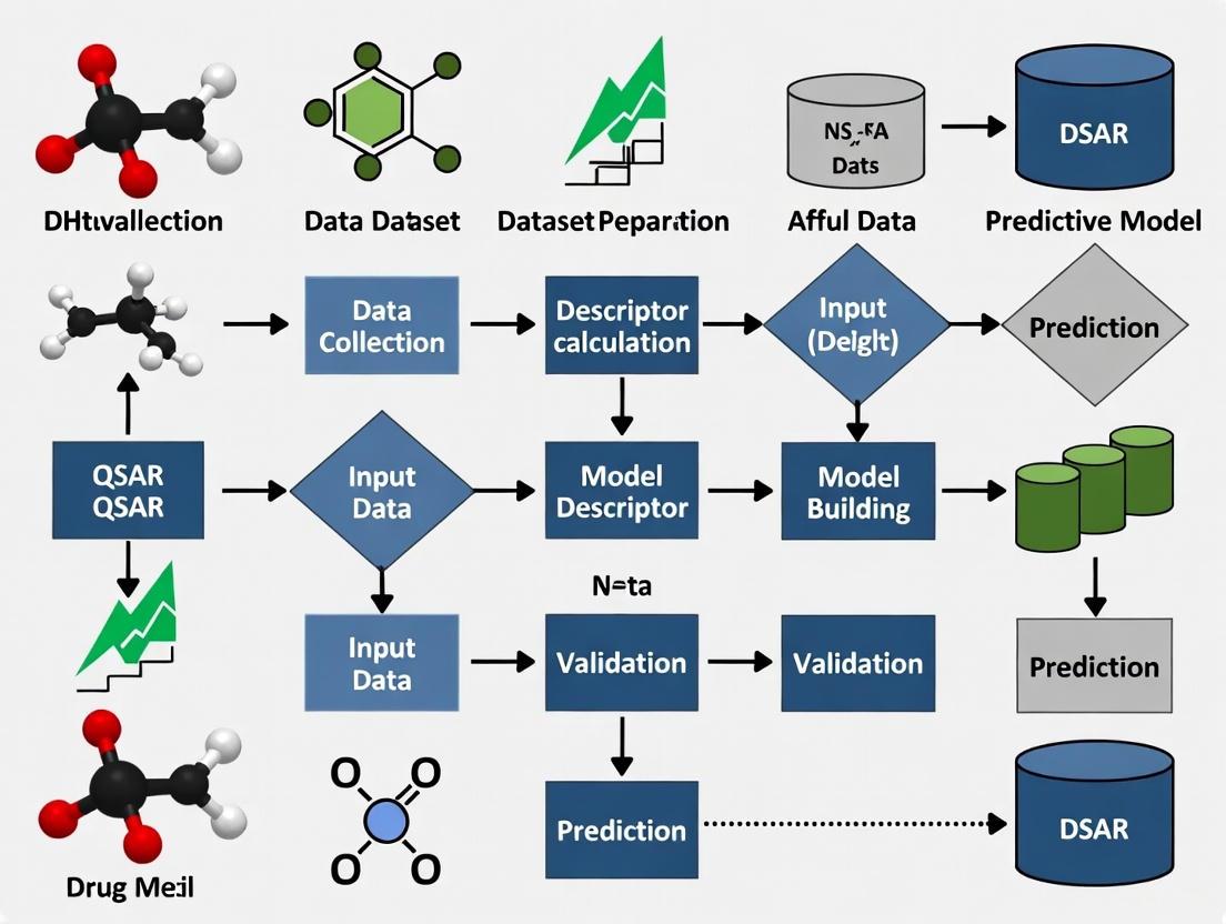
Diagram 1: QSAR Model Development Workflow. This flowchart outlines the standard procedure for developing validated QSAR models, from initial data collection through to final predictive application.
Application Note: QSAR in Anti-Malarial Drug Discovery
Experimental Background and Objectives
The emergence of artemisinin resistance in Plasmodium falciparum has created an urgent need for novel antimalarial agents with new mechanisms of action [8]. Dihydroorotate dehydrogenase (DHODH) represents a promising drug target as it catalyzes a critical step in pyrimidine biosynthesis essential for parasite proliferation [8]. This application note details a QSAR study aimed at developing predictive classification models for identifying novel PfDHODH inhibitors, demonstrating the practical implementation of the QSAR paradigm in addressing a significant public health challenge.
Detailed Experimental Protocol
Data Set Curation and Preparation
- Data Source: IC~50~ values for PfDHODH inhibitors were extracted from the ChEMBL database (ChEMBL ID CHEMBL3486), a manually curated repository of bioactive molecules with drug-like properties [8].
- Data Curation: The initial data set was rigorously curated to remove duplicates, compounds with missing activity values, and those falling outside relevant potency ranges. This resulted in a final set of 465 inhibitors for model development [8].
- Activity Classification: Continuous IC~50~ values were converted to categorical classes (active/inactive) using appropriate threshold values based on biological significance.
- Data Splitting: The curated data set was divided into training (~80%) and external test (~20%) sets using statistical methods such as Kennard-Stone algorithm to ensure representative chemical space coverage [8] [6].
Molecular Descriptor Calculation and Feature Selection
- Descriptor Types: Twelve distinct sets of chemical fingerprints (binary structural keys representing molecular features) were calculated for all compounds using cheminformatics software [8].
- Feature Selection: Recursive feature elimination was employed to identify the most informative molecular descriptors, removing 62-99% of redundant features to reduce noise and prevent model overfitting [8] [9].
- Data Balancing: Both undersampling and oversampling techniques were applied to address class imbalance, with balanced oversampling proving most effective for this data set [8].
Model Building and Optimization
- Algorithm Selection: Twelve different machine learning algorithms were evaluated, including Random Forest (RF), Support Vector Machines (SVM), and Neural Networks [8].
- Hyperparameter Tuning: Model hyperparameters were optimized via grid search with 5-fold cross-validation on the training set to maximize predictive performance [8].
- Model Training: Final models were trained using the optimized parameters on the complete training set.
Model Validation and Evaluation
- Internal Validation: Model performance was assessed via cross-validation on the training set using Matthew's Correlation Coefficient (MCC) as the primary metric [8].
- External Validation: The final model was evaluated on the held-out test set to estimate real-world predictive performance [8] [6].
- Applicability Domain: The chemical space where the model could make reliable predictions was characterized to guide appropriate application [10].
Key Results and Research Implications
The optimized Random Forest model using SubstructureCount fingerprints demonstrated superior performance with MCC values of 0.97 (training), 0.78 (cross-validation), and 0.76 (external test set), indicating high predictive accuracy and robustness [8]. Feature importance analysis using the Gini index revealed that nitrogenous groups, fluorine atoms, oxygen-containing functionalities, aromatic moieties, and chirality centers were critical structural features influencing PfDHODH inhibitory activity [8].
This QSAR study successfully identified key structural determinants for PfDHODH inhibition, providing valuable insights for medicinal chemistry optimization of lead compounds. The validated model enables virtual screening of compound libraries to identify novel chemotypes with potential anti-malarial activity, significantly accelerating the drug discovery process against artemisinin-resistant malaria [8].
Advanced Protocols in QSAR Modeling
Comprehensive Model Validation Framework
Robust validation is imperative for developing reliable QSAR models with true predictive power [1] [6]. The following multi-tiered validation protocol must be implemented:
Table 2: Comprehensive QSAR Model Validation Strategy
| Validation Type | Protocol | Key Metrics | Acceptance Criteria |
|---|---|---|---|
| Internal Validation | 5-fold or 10-fold cross-validation | Q², R², RMSE | Q² > 0.6 for regression; MCC > 0.6 for classification |
| External Validation | Prediction on completely held-out test set | Predictive R², Concordance | R²~pred~ > 0.6; Strong correlation (p < 0.05) |
| Randomization Test | Y-scrambling with multiple iterations | R²~random~, Q²~random~ | Significant difference from original model (p < 0.01) |
| Applicability Domain | Leverage approaches, distance measures | Williams plot, PCA-based distance | >80% of predictions within domain |
Internal validation via cross-validation assesses model robustness by iteratively partitioning the training data and measuring predictive performance across folds [6]. External validation using a completely independent test set provides the most realistic estimate of a model's predictive power for novel compounds [6]. Y-randomization tests confirm that model performance stems from genuine structure-activity relationships rather than chance correlations [1]. Defining the applicability domain is crucial for identifying the chemical space where the model can make reliable predictions [10].
Table 3: Essential Computational Tools for QSAR Modeling
| Tool Category | Representative Software/Services | Primary Function | Key Features |
|---|---|---|---|
| Descriptor Calculation | PaDEL-Descriptor, Dragon, RDKit, Mordred | Generate molecular descriptors from structures | 1D-3D descriptors, fingerprint generation, batch processing |
| Cheminformatics Platforms | KNIME, Orange, Pipeline Pilot | Workflow automation and data pipelining | Visual programming, data preprocessing, model integration |
| Machine Learning Libraries | Scikit-learn, TensorFlow, PyTorch | Algorithm implementation and model building | Extensive algorithm collections, neural networks, hyperparameter optimization |
| Chemical Databases | ChEMBL, PubChem, ZINC | Source of chemical structures and bioactivity data | Annotated bioactivities, commercial availability, structural diversity |
| Model Validation Suites | QSAR Model Reporting Format (QMRF), OECD QSAR Toolbox | Standardized model validation and reporting | Regulatory compliance, standardized metrics, interoperability |
Deep QSAR and Emerging Methodologies
The integration of deep learning with traditional QSAR has created the emerging subfield of "deep QSAR" [5]. These approaches leverage neural networks with multiple hidden layers to automatically learn relevant feature representations from molecular structures, potentially surpassing the predictive performance of traditional descriptor-based methods [5] [7].
Advanced deep QSAR protocols include:
- Graph Neural Networks that operate directly on molecular graphs, inherently capturing topological relationships [5]
- Multi-task learning frameworks that simultaneously predict multiple biological endpoints, leveraging shared representations across related tasks [5]
- Hybrid models integrating QSAR with molecular dynamics simulations to incorporate structural and dynamical information [7]
- Generative models for de novo molecular design that create novel chemical structures with optimized properties [5]
Diagram 2: Comparison of Traditional and Deep QSAR Approaches. This diagram contrasts descriptor-based QSAR, which relies on pre-calculated molecular features, with deep QSAR methods that automatically learn relevant representations from raw molecular inputs.
The QSAR paradigm has evolved from simple linear regression models based on handfuls of interpretable descriptors to complex, high-dimensional models capable of predicting diverse biological endpoints with remarkable accuracy [4]. This evolution has been driven by advances in three critical areas: the emergence of larger, higher-quality datasets; the development of more sophisticated molecular descriptors; and the adoption of powerful machine learning algorithms, particularly deep learning architectures [5] [4].
Future developments in QSAR modeling will likely focus on expanding applicability domains to encompass more diverse chemical space, improving model interpretability through explainable AI techniques, and enhancing predictive reliability for novel chemotypes [4]. The integration of QSAR with structural biology information through hybrid approaches, along with the adoption of multi-task and transfer learning strategies, promises to further increase the utility of these models in drug discovery pipelines [7]. As these methodologies continue to mature, QSAR will remain an indispensable component of the molecular design toolkit, enabling more efficient exploration of chemical space and acceleration of therapeutic development.
In the disciplined pursuit of drug discovery, Quantitative Structure-Activity Relationship (QSAR) modeling serves as a fundamental in silico technique that correlates the structural properties of molecules with their biological activity [11]. The predictive power and interpretability of these models are wholly dependent on the molecular descriptors used as input variables. Molecular descriptors are numerical quantities that encode chemical information derived from a molecule's symbolic representation, transforming molecular structures into useful numbers for computational analysis [12] [13].
The selection of appropriate descriptors is therefore not merely a preliminary step but a critical decision point that dictates the success of any QSAR workflow. Descriptors span multiple levels of complexity—from simple atomic counts to sophisticated quantum mechanical calculations—each capturing different facets of molecular structure and properties [13] [14]. This article provides a structured overview of essential molecular descriptors across this complexity spectrum, presents practical protocols for their application, and integrates this knowledge within a comprehensive QSAR model development framework, empowering researchers to make informed choices in their molecular design efforts.
A Hierarchical Taxonomy of Molecular Descriptors
Molecular descriptors can be systematically classified based on the dimensionality of the molecular representation from which they are derived and the chemical information they encode. This hierarchical taxonomy progresses from simple, easily computed descriptors to complex, information-rich ones, with each category serving distinct purposes in QSAR modeling [13] [14].
Table 1: Classification of Molecular Descriptors by Dimensionality and Type
| Descriptor Class | Information Content | Key Examples | Typical QSAR Application |
|---|---|---|---|
| 0D (Constitutional) | Atomic composition & counts; additive properties | Molecular weight, atom counts, molecular formula [13] [14] | Preliminary screening, drug-likeness filters (e.g., Lipinski's Rule of 5) |
| 1D (Substructural) | Presence/absence or count of specific fragments | Functional group counts, hydrogen bond donors/acceptors, rotatable bonds [13] | Pharmacophore feature identification, toxicity prediction |
| 2D (Topological) | Atomic connectivity & molecular graph features | Wiener index, Zagreb index, connectivity indices, Kier & Hall descriptors [11] [12] | High-throughput virtual screening, similarity searching |
| 3D (Geometric/Steric) | 3D atomic coordinates & spatial arrangement | Molecular volume, surface area, 3D-MoRSE descriptors, WHIM descriptors [12] [13] | Modeling stereoselective interactions, receptor fit prediction |
| 3D (Quantum Chemical) | Electronic distribution & energetics | Partial atomic charges, HOMO/LUMO energies, dipole moment, polarizability [15] [16] | Modeling electronic-driven interactions, reaction mechanism studies |
| 4D (Interaction Fields) | Ligand-probe interaction energies in 3D space | GRID, CoMFA, CoMSIA fields [13] [14] | Detailed structure-based design, understanding binding interactions |
The foundational principle when selecting descriptors is that the information content of the descriptors should be appropriately matched to the complexity of the biological endpoint being modeled [13]. Using overly simplistic descriptors for a complex phenomenon may yield uninformative models, while using highly complex descriptors for a simple property may introduce noise and lead to overfitting [11] [13]. The following sections detail the primary descriptor classes within this hierarchy.
0D and 1D Descriptors: The Constitutional and Substructural Foundation
0D descriptors are derived from the chemical formula alone and require no information about molecular structure or connectivity [13]. They include simple counts of atoms and bonds, molecular weight, and sums of basic atomic properties. While their information content is low and they often have high degeneracy (the same value for different molecules, including isomers), they are straightforward to calculate, interpret, and are invaluable for constructing simple, robust models for properties like molecular refractivity [13].
1D descriptors incorporate substructural information, typically representing the presence, absence, or frequency of specific functional groups or fragments in a molecule [13]. These include counts of hydrogen bond donors and acceptors, rotatable bonds (a measure of flexibility), and rings. Such descriptors form the basis of popular drug-likeness rules and are essential in substructural analysis for identifying toxicophores or other activity-defining fragments [17].
2D Descriptors: Harnessing the Power of Molecular Topology
2D descriptors, or topological indices, are derived from the hydrogen-suppressed molecular graph, where atoms are represented as vertices and bonds as edges [11] [13]. They encode patterns of atomic connectivity and are invariant to the molecule's conformation. Key categories include:
- Connectivity Indices (e.g., Randić, Kier & Hall): These capture the degree of branching in a molecule and have been successfully correlated with various physicochemical properties [11].
- Wiener Index: One of the earliest topological indices, defined as the sum of the shortest path distances between every pair of atoms in the molecular graph, related to molecular volume and boiling points [11].
- Kappa Shape Indices: Describe the molecular shape and flexibility based on the graph's topology [11].
A significant advantage of 2D descriptors is their computational efficiency and independence from molecular conformation, making them ideal for high-throughput screening of large chemical databases [11] [14]. In many practical applications, models built with 2D descriptors perform as well as, or even better than, those built with more complex 3D descriptors [14].
3D Descriptors: Encoding Spatial and Electronic Reality
3D descriptors require the 3D spatial coordinates of a molecule's atoms and thus capture stereochemical and geometric information that 2D descriptors cannot [13]. This class can be further divided into steric/geometric and quantum chemical descriptors.
Steric and Geometric Descriptors include simple measures like molecular volume, solvent-accessible surface area, and moment of inertia, which describe the overall size and shape of the molecule [17]. More sophisticated 3D descriptors, such as WHIM (Weighted Holistic Invariant Molecular) and 3D-MoRSE (3D Molecule Representation of Structures based on Electron diffraction), are holistic representations that are invariant to translation and rotation [12] [13].
Quantum Chemical Descriptors are derived from quantum mechanical calculations and provide detailed insight into a molecule's electronic structure and reactivity [15] [16]. Key descriptors include:
- HOMO/LUMO Energies: The energies of the Highest Occupied and Lowest Unoccupied Molecular Orbitals, indicating a molecule's ability to donate or accept electrons.
- Partial Atomic Charges: Describe the electron density distribution and are critical for modeling electrostatic interactions.
- Dipole Moment and Polarizability: Measure the overall molecular polarity and its response to an electric field.
These descriptors are indispensable for modeling biological activities where electronic effects, such as charge-transfer interactions or covalent binding, play a dominant role [16]. Their calculation, however, is computationally intensive and requires careful geometry optimization [15].
4D Descriptors and Beyond: Capturing Interaction Landscapes
4D descriptors extend the concept further by incorporating interaction energy information within a 3D grid. In methods like GRID, CoMFA (Comparative Molecular Field Analysis), and CoMSIA (Comparative Molecular Similarity Indices Analysis), the molecule is placed in a 3D lattice, and its interaction energies with various chemical probes (e.g., water, methyl group, carbonyl oxygen) are computed at each grid point [13] [14]. This rich data captures the molecule's potential interaction preferences with a biological target, providing a direct link to structure-based design principles.
Diagram 1: A strategic workflow for selecting molecular descriptors within a QSAR model development pipeline, highlighting key decision points.
Essential Protocols for Descriptor Calculation and Selection
Protocol 1: Calculation of a Comprehensive 2D Descriptor Set Using RDKit
Objective: To compute a diverse set of 2D molecular descriptors (constitutional, topological, and electronic) directly from SMILES strings using the open-source RDKit library.
Materials:
- Software: Python environment with RDKit installed.
- Input Data: A file containing molecular structures as SMILES strings and a corresponding compound identifier.
Procedure:
- Environment Setup: Install the RDKit library via conda (
conda install -c conda-forge rdkit). - Data Loading: Read the input file (e.g., CSV) using pandas.
- Molecule Object Generation: Iterate through the SMILES strings and convert each into an RDKit molecule object. Include sanitization checks to handle invalid structures.
- Descriptor Calculation: Utilize RDKit's descriptor modules (
rdkit.Chem.Descriptorsandrdkit.ML.Descriptors) to calculate a comprehensive set of properties. Key descriptors to include are:- Constitutional: Molecular weight, number of heavy atoms, rotatable bonds, H-bond donors/acceptors.
- Topological: Topological polar surface area (TPSA), graph-based indices.
- Electronic: Crippen logP and molar refractivity.
- Data Output: Compile all calculated descriptors into a structured data frame and export to a CSV file for subsequent modeling.
Notes: This protocol is highly efficient for large datasets. RDKit computes these descriptors from the 2D graph, requiring no 3D conformation, which makes it exceptionally fast [14].
Protocol 2: Feature Selection Using VSURF in a QSAR Workflow
Objective: To identify a non-redundant, biologically relevant subset of descriptors from a large initial pool to build a robust, interpretable, and predictive QSAR model while avoiding overfitting.
Materials:
- Software: R statistical environment with the
VSURFpackage installed. (Note: This method is also integrated into automated workflow tools like the KNIME-based workflow cited [18]). - Input Data: A data matrix where rows are compounds and columns are the extensive set of calculated molecular descriptors and the corresponding biological activity values.
Procedure:
- Data Preprocessing: Clean the descriptor matrix by removing descriptors with near-zero variance or high pairwise correlation.
- VSURF Execution: Run the
VSURFfunction, which is a Random Forest-based algorithm that operates in three steps [18]:- Step 1 (Interpretation): Eliminates descriptors irrelevant to the activity.
- Step 2 (Prediction): Selects a small subset of descriptors that contribute meaningfully to prediction accuracy.
- Step 3 (Selection): Removes redundant descriptors from the subset obtained in Step 2.
- Output Analysis: The final output of VSURF is a minimal set of descriptors that are most predictive. The relative importance of these descriptors should be examined to gain mechanistic insights.
Notes: Feature selection is a critical step in QSAR model development. It improves model interpretability, reduces the risk of overfitting from noisy descriptors, and can provide faster and more cost-effective models [11] [18].
Table 2: Key Software Tools for Molecular Descriptor Calculation
| Tool Name | Descriptor Coverage | Key Features | License |
|---|---|---|---|
| alvaDesc [12] | 0D to 3D, Fingerprints | Comprehensive, user-friendly GUI & CLI, updated in 2025 | Commercial |
| Dragon [12] [17] | 0D to 3D, >5000 descriptors | Historically a gold standard, now discontinued | Was Commercial |
| RDKit [12] [17] | 0D, 2D, 3D, Fingerprints | Open-source, Python API, active development, highly customizable | Free Open Source |
| Mordred [12] | 0D, 2D, 3D | Open-source, based on RDKit, calculates >1800 descriptors, Python library | Free Open Source |
| PaDEL-Descriptor [12] [17] | 0D, 2D, 3D, Fingerprints | Based on the Chemistry Development Kit (CDK), GUI and CLI, now discontinued | Free |
The Scientist's Toolkit: Research Reagent Solutions
Table 3: Essential Computational Tools for a QSAR Workflow
| Tool / Resource | Category | Function in QSAR Workflow |
|---|---|---|
| RDKit [12] [17] | Cheminformatics Library | Core calculation of 2D/3D descriptors and fingerprints; molecule handling. |
| VSURF R Package [18] | Feature Selection Algorithm | Identifies relevant, non-redundant descriptors from a large initial pool. |
| KNIME Analytics Platform [18] | Workflow Management | Provides a visual interface to build, execute, and manage the entire QSAR pipeline. |
| alvaDesc [12] | Descriptor Software | Computes a vast array of 0D-3D descriptors for robust model development. |
| SYNTHIA Retrosynthesis [19] | Synthesis Planning | Aids in the design of synthetically accessible compounds identified via QSAR. |
Concluding Remarks
The strategic selection of molecular descriptors is a cornerstone of effective QSAR model development. As explored throughout this article, the descriptor landscape is hierarchically structured, ranging from fast-computing constitutional descriptors to mechanistically insightful quantum chemical indices. The guiding principle for the modeler is to align the complexity of the descriptors with the specific biological endpoint and the project's goals, whether it be high-throughput virtual screening or detailed mechanistic elucidation [11] [13].
The future of descriptors in QSAR is being shaped by the integration of artificial intelligence and machine learning. Recent research focuses on developing methods for the dynamic adjustment of descriptor importance [20] and on leveraging deep learning to automatically derive optimal molecular representations from raw structural data [17]. Furthermore, the push for model interpretability remains paramount, as evidenced by the OECD's principle that QSAR models should have a mechanistic interpretation, wherever possible [20]. By thoughtfully applying the protocols and principles outlined in this article, researchers can harness the full power of molecular descriptors to accelerate the rational design of novel, effective therapeutics.
Within the Quantitative Structure-Activity Relationship (QSAR) model development workflow, the initial stages of data collection and curation are not merely preliminary steps but are fundamentally critical to the success and reliability of any subsequent computational analysis. The principle of "garbage in, garbage out" is acutely relevant; even the most sophisticated machine learning algorithms cannot compensate for poor-quality input data [21]. Robust data collection and curation strategies ensure that the developed models are predictive, interpretable, and suitable for regulatory acceptance. These processes involve gathering relevant chemical structures and their associated biological activities, followed by a rigorous protocol to check their correctness, standardize them, and produce consistent, ready-to-use datasets for cheminformatic analysis [22]. This document outlines detailed application notes and protocols for these foundational stages, framed within the broader context of a QSAR model development thesis.
The Critical Role of Data Quality in QSAR
The evolution of QSAR from basic linear models to advanced machine learning and AI-based techniques has placed an even greater emphasis on dataset quality, reproducibility, and the clear definition of a model's applicability domain [21]. High-quality, well-curated data is the bedrock upon which robust, predictive models are built. Inadequate attention to data quality at this stage can introduce biases and errors that propagate through the entire workflow, leading to models with poor predictive performance and limited practical utility. Furthermore, regulatory guidelines, such as those from the OECD, emphasize the importance of reliable data for ensuring model credibility in chemical safety and pharmaceutical applications [21]. A standard procedure for data retrieval and curation, implemented in freely available workflows, has been recognized as a tool of high interest in the field of computational chemistry [22].
Consequences of Inadequate Data Curation
Neglecting rigorous data curation can lead to several critical failures in QSAR modeling:
- Introduction of Biases and Errors: Incorrect structures or inconsistent activity data can skew the model's learning process.
- Poor Predictive Performance: Models built on unreliable data fail to generalize to new, external chemicals.
- Limited Regulatory Acceptance: Models that do not adhere to best practices for data quality, as outlined in OECD guidelines, are unlikely to be accepted for regulatory decision-making [21].
- Misleading Structure-Activity Relationships: The core objective of the model is compromised, leading to incorrect hypotheses about the chemical features responsible for biological activity.
Data Collection and Curation Protocol
The following protocol provides a detailed methodology for the collection and curation of chemical data to develop a high-quality dataset for QSAR modeling. The entire workflow is also summarized in Figure 1.
Data Collection and Acquisition
Objective: To gather a comprehensive set of chemical structures and their corresponding biological activity data from reliable public and/or proprietary sources.
Materials and Reagents:
- Public Chemical Databases: (e.g., PubChem, ChEMBL). Provide a rich source of bioactive molecules and their properties.
- Proprietary Corporate Databases: Internal collections of synthesized and tested compounds.
- Literature Mining Tools: Software to extract chemical and biological data from scientific publications.
Procedure:
- Define Scope and Endpoint: Clearly delineate the chemical space and the biological activity or toxicity endpoint of interest (e.g., IC50, LD50). This defines the model's applicability domain from the outset [21].
- Identify Data Sources: Select appropriate public and/or proprietary databases from which to retrieve chemical data, typically in the form of SMILES (Simplified Molecular-Input Line-Entry System) strings [22].
- Data Retrieval: Extract chemical structures (as SMILES, SDF, or other formats) and their associated experimental endpoint values. Ensure that all data is associated with consistent units of measurement.
Data Curation and Standardization
Objective: To check the correctness of the retrieved chemical data and curate them to produce a consistent and ready-to-use dataset [22].
Procedure:
- Structure Verification:
- Check the validity of all SMILES strings or structural files.
- Remove any entries that contain atoms other than those in the defined set (e.g., no heavy metals for a drug-like dataset).
- Check and correct for valency errors.
- Standardization (See Table 1 for common tasks):
- Tautomer Standardization: Select a single, representative tautomer for each molecule to ensure consistency.
- Charge Standardization: Standardize protonation states to a relevant pH (e.g., pH 7.4) using appropriate tools.
- Stereochemistry: Define and consistently represent stereochemical centers. Consider defining racemic mixtures explicitly if the experimental data does not distinguish enantiomers.
- Descriptor Calculation: Use open-source software like PaDEL-Descriptor to calculate molecular descriptors and fingerprints [21].
- Activity Data Verification:
- Unit Consistency: Ensure all biological activity values (e.g., IC50, Ki) are reported in the same unit (e.g., nM, µM).
- Duplicate Removal: Identify and resolve duplicate entries for the same chemical structure. Prefer the most reliable measurement or calculate an average if multiple valid measurements exist.
- Outlier Detection: Visually and statistically inspect the distribution of activity values to identify and investigate potential outliers that may represent experimental errors. The use of binned histograms can be highly effective for visual outlier detection [23].
Dataset Preparation for Modeling
Objective: To create the final, curated dataset that is partitioned for model training and validation.
Procedure:
- Chemical Diversity Analysis: Assess the structural diversity of the curated dataset using calculated descriptors to ensure a representative coverage of the chemical space.
- Data Splitting: Split the curated dataset into training and test sets using methods such as random splitting or time-split cross-validation [21]. This is critical for estimating the goodness of prospective prediction.
- Format for Analysis: Structure the data into a single, well-formatted table. As a fundamental best practice for analysis, each row should represent a unique compound, and each column should represent an attribute of that compound, such as a descriptor or the activity value [23]. Ensure the data is stored in rows and columns, with column headers in the first row.
Figure 1: Data Curation Workflow. This diagram outlines the logical sequence of steps for curating chemical data for QSAR modeling.
Data Presentation and Analysis
This section summarizes key quantitative aspects and reagent solutions involved in the data curation process for easy comparison and implementation.
Table 1: Common Data Standardization Tasks in QSAR Curation
| Standardization Task | Description | Common Tools/Functions |
|---|---|---|
| Tautomer Standardization | Selects a single, representative tautomeric form for each molecule to ensure consistency. | RDKit (CanonicalTautomer), OpenBabel |
| Charge Standardization | Adjusts protonation states to a defined pH (e.g., 7.4) to reflect physiological conditions. | RDKit, MOE, ChemAxon Marvin |
| Stereochemistry Definition | Explicitly defines stereocenters; important for chiral activity differences. | RDKit, CDK (Chemistry Development Kit) |
| Descriptor Calculation | Generates numerical representations of molecular structures. | PaDEL-Descriptor [21], RDKit, Dragon |
| Duplicate Removal | Identifies and consolidates or removes identical chemical structures. | In-house scripts, KNIME, Pipeline Pilot |
Table 2: Essential Research Reagent Solutions for QSAR Data Curation
| Item / Solution | Function / Purpose |
|---|---|
| KNIME Analytics Platform | An open-source platform for implementing automated workflows for data retrieval, curation, and machine learning in QSAR [22]. |
| RDKit | An open-source cheminformatics toolkit used for molecule standardization, descriptor calculation, and scaffold analysis. |
| PaDEL-Descriptor Software | Open-source software to calculate a comprehensive set of molecular descriptors and fingerprints [21]. |
| Public Chemical Databases (e.g., ChEMBL, PubChem) | Provide large, annotated chemical datasets of bioactive molecules for model building. |
| Curated In-House Compound Libraries | Proprietary collections of chemically diverse compounds with high-quality, internally generated activity data. |
The development of robust Quantitative Structure-Activity Relationship (QSAR) models fundamentally depends on the quality and consistency of the underlying chemical structure input. The concept of "QSAR-ready" structures describes chemical representations that have undergone standardized preparation to ensure molecular descriptors calculated from them accurately reflect the compounds' properties and biological activities. This process is particularly critical for tautomerizable molecules, which constitute approximately 25% of marketed drugs and can exist as multiple structures interconverting through proton movement and bond rearrangement [24] [25]. Without proper standardization, the same compound represented in different tautomeric states can yield different molecular fingerprints, hydrophobicities, pKa values, and three-dimensional shapes, ultimately compromising QSAR model accuracy, repeatability, and reliability [26] [24].
This application note details standardized protocols for achieving QSAR-ready chemical structures through automated standardization workflows with particular emphasis on tautomer handling. Framed within the broader context of QSAR model development workflow research, we provide comprehensive methodologies, practical tools, and validation approaches to ensure chemical data quality prior to model building.
The Critical Challenge of Tautomerism in QSAR
Prevalence and Impact on Modeling
Tautomerism presents a multifaceted challenge for computer-aided molecular design. Analysis of marketed drugs reveals that 26% exist as an average of three tautomers, potentially increasing dataset size by 1.64-fold when all forms are considered [24]. Different tautomers of the same molecule exhibit distinct molecular fingerprints, hydrophobicities, pKa values, 3D shapes, and electrostatic properties [24]. Furthermore, proteins frequently preferentially bind to a tautomer that may be present in low abundance in aqueous solution, creating discrepancies between experimental conditions and computational representations [24].
The proper treatment of tautomers affects virtually every aspect of QSAR modeling:
- Library Design: Similarity or diversity assessments may inadvertently include similar molecules encoded as different tautomers
- Descriptor Calculation: QSAR algorithms must decide which tautomer(s) to use for molecular descriptor calculation
- Model Interpretation: Structure-activity relationships become complicated when tautomerism influences biological activity measurements
- Virtual Screening: Docking protocols must determine which tautomers to include and account for tautomerization in scoring functions [24]
Thermodynamic Considerations and Environmental Dependence
Tautomeric ratios are highly dependent on molecular structure and solvent environment [24]. Small changes in structure or solvent can dramatically alter tautomer distributions, complicating the assignment of physical property measurements to specific chemical structures and identification of bioactive species from tautomeric mixtures. Table 1 summarizes key factors influencing tautomeric equilibria.
Table 1: Factors Influencing Tautomeric Equilibria
| Factor | Impact on Tautomerism | Example |
|---|---|---|
| Solvent Environment | Dramatically shifts tautomer ratios | 4-Hydroxypyridine exists predominantly as 4-pyridone in water [24] |
| Substituent Effects | Electronic properties influence preferred form | Ortho-nitro group favors open form in ring-chain tautomerism [24] |
| Intramolecular H-bonding | Can stabilize otherwise less favored tautomers | Intramolecular H-bonds in enol forms can increase their prevalence [24] |
| Protein Binding | Macromolecules may selectively bind minor tautomers | Barbiturate analogue bound to matrix metalloproteinase 8 as minor tautomer (20 kcal/mol less stable in solution) [24] |
| Measurement Context | Experimental conditions affect observed ratios | NMR may detect multiple tautomers while crystallography might capture only one [24] |
Automated Workflows for QSAR-Ready Standardization
Comprehensive Standardization Protocol
The "QSAR-ready" workflow represents a systematic approach to chemical structure standardization prior to QSAR modeling. Implemented within the KNIME workflow environment, this automated protocol ensures consistent molecular representations across diverse chemical datasets [26]. The workflow comprises three high-level steps:
- Structure Encoding and Reading: Chemical structures are read from various input formats and converted into in-memory molecular representations
- Identifier Cross-Referencing: Existing chemical identifiers are cross-referenced for consistency verification
- Structure Standardization: A series of operations transforms structures into standardized representations [26]
The following diagram illustrates the complete QSAR-ready standardization workflow:
Tautomer Handling Methodologies
Tautomer standardization represents perhaps the most critical step in the QSAR-ready workflow. Multiple approaches exist for addressing tautomerism in computational chemistry, each with distinct advantages and limitations:
Rule-Based Tautomer Standardization
Most automated QSAR workflows implement rule-based systems that transform tautomers into a single canonical representation. These systems typically:
- Enumerate possible tautomers based on molecular structure
- Apply predetermined rules to select the predominant tautomer
- Generate standardized output for descriptor calculation [26]
This approach balances computational efficiency with reasonable accuracy for most QSAR applications, particularly when processing large chemical datasets.
Quantum Mechanical Approaches
For higher accuracy requirements, quantum mechanics (QM) based methods provide a more rigorous foundation for tautomer prediction. These approaches calculate the relative energies of different tautomers to determine their stability and prevalence. Traditional QM methods like Density Functional Theory (DFT) calculations offer accuracy but remain computationally prohibitive for large datasets [25].
Emerging hybrid quantum chemistry-quantum computation workflows show promise for efficient prediction of preferred tautomeric states. These approaches:
- Select active-space molecular orbitals based on quantum chemistry methods
- Map Hamiltonian onto quantum devices using efficient encoding methods
- Employ variational quantum eigensolver (VQE) algorithms for ground state estimation [25]
While still in development, quantum computing approaches may eventually enable accurate tautomer prediction with reduced computational resources compared to traditional QM methods [25].
Experimental Protocols and Implementation
Protocol: QSAR-Ready Standardization in KNIME
This protocol details the implementation of an automated QSAR-ready workflow using KNIME analytics platform [26]:
Materials:
- Chemical structures in SMILES, SDF, or other standard formats
- KNIME Analytics Platform (version 4.0 or higher)
- CDK (Chemistry Development Kit) nodes or RDKit nodes within KNIME
- "QSAR-ready" workflow components [26]
Procedure:
- Data Input Configuration
- Configure file reader nodes to import chemical structures
- Specify input format (SMILES, SDF, etc.) and character encoding
- Include appropriate identifier fields for cross-referencing
Structure Standardization
- Implement desalting step to remove counterions and salts
- Apply stereochemistry stripping for 2D QSAR models
- Configure tautomer standardization parameters:
- Set maximum number of tautomers to generate (default: 100)
- Define reaction patterns for proton movement
- Specify timeout for tautomer enumeration (default: 60 seconds)
- Apply nitro group standardization to consistent representations
- Implement valence correction to fix invalid valence states
- Configure neutralization rules for ionizable groups
Duplicate Handling
- Set similarity threshold for duplicate identification (typically 0.95-1.0 Tanimoto)
- Define precedence rules for duplicate selection (e.g., highest data quality)
- Implement duplicate removal or grouping
Output Generation
- Export standardized structures in desired format
- Include audit trail of applied transformations
- Generate summary statistics of standardization results
Validation:
- Compare molecular descriptor variance before and after standardization
- Verify consistent representation of known tautomer pairs
- Assess impact on QSAR model performance using control datasets
Protocol: Tautomer Enumeration and Scoring
For applications requiring explicit consideration of multiple tautomeric states, this protocol describes a comprehensive tautomer handling approach:
Materials:
- Chemical structure with tautomerizable functional groups
- Tautomer enumeration software (e.g., ChemAxon, OpenEye)
- Computational resources for quantum mechanical calculations (optional)
Procedure:
- Tautomer Enumeration
- Identify tautomerizable functional groups (keto-enol, lactam-lactim, etc.)
- Generate all possible tautomers considering:
- Proton movement between heteroatoms
- Ring-chain equilibria
- Valence tautomerism
- Apply ring conformation analysis where relevant
Tautomer Scoring
- Method A: Empirical Scoring
- Apply rule-based prioritization (e.g., favor keto over enol forms)
- Use known thermodynamic preferences for common scaffolds
- Consider steric and electronic effects of substituents
- Method B: Quantum Mechanical Scoring
- Perform geometry optimization for each tautomer
- Calculate relative energies using appropriate theory level (e.g., B3LYP/6-31G*)
- Include solvation effects using implicit solvent models (e.g., PCM, SMD)
- Apply Boltzmann distribution to estimate population ratios
- Method A: Empirical Scoring
Representation Selection
- For single-representation QSAR: Select lowest energy tautomer
- For multi-representation QSAR: Include all tautomers above population threshold (e.g., >5%)
- Weight contributions according to estimated populations if needed
Validation:
- Compare predicted dominant tautomers with experimental crystal structures where available
- Validate population estimates against spectroscopic data
- Assess consistency across different enumeration algorithms
Essential Tools for QSAR-Ready Standardization
The Scientist's Toolkit: Software Solutions
Table 2: Essential Tools for Achieving QSAR-Ready Chemical Structures
| Tool Name | Type | Key Features | Tautomer Handling | License |
|---|---|---|---|---|
| KNIME with Chemistry Extensions | Workflow Platform | Automated QSAR-ready workflow, visual pipeline design, descriptor calculation [26] | Rule-based standardization with customizable parameters | Open Source |
| QSPRpred | Python Package | Data set curation, model building, serialization of preprocessing steps [27] | Integration with external tautomer standardization libraries | Open Source |
| QSAR Toolbox | Comprehensive Application | Data gap filling, metabolic simulation, read-across, category building [28] | Integrated tautomer profiling and metabolism simulation | Free |
| PaDEL-Descriptor | Descriptor Calculator | Molecular descriptor and fingerprint calculation, includes pre-processing [29] | Basic structure standardization prior to descriptor calculation | Open Source |
| Epik | Tautomer Prediction | pKa prediction, tautomer enumeration, ligand preparation for docking | Physics-based methods for tautomer population estimation | Commercial |
Implementation Considerations for Automated Workflows
When implementing automated QSAR-ready workflows, several critical factors ensure success:
Data Quality Assessment:
- Evaluate dataset modelability before extensive processing
- Identify potential representation inconsistencies early
- Establish baseline quality metrics for comparison [9]
Feature Selection Integration:
- Implement efficient variable selection to remove redundant descriptors
- Reduce prediction error by 19% on average through proper feature selection
- Increase percentage of variance explained (PVE) by 49% compared to models without feature selection [9]
Reproducibility and Deployment:
- Serialize complete preprocessing workflows alongside models
- Ensure consistent application of standardization to new compounds
- Document all transformation parameters for regulatory compliance [27]
Impact on QSAR Model Performance
Proper structure standardization significantly enhances QSAR model reliability. Studies demonstrate that automated QSAR-ready workflows:
- Improve model accuracy through consistent molecular representation
- Enhance model reproducibility across different research groups
- Increase descriptor reliability by eliminating representation artifacts [26]
For tautomer-rich datasets, appropriate handling can determine model success. Comparative studies show that models built with standardized tautomer representations outperform those using raw chemical inputs, particularly for endpoints sensitive to hydrogen bonding and molecular shape [24].
Achieving QSAR-ready structures through automated standardization and systematic tautomer handling represents a foundational step in robust QSAR model development. The protocols and methodologies detailed in this application note provide researchers with practical approaches to address chemical representation challenges, particularly for the approximately 25% of drug-like molecules capable of tautomerism.
Future developments in this field will likely include:
- Increased integration of quantum mechanical methods for tautomer prediction
- Hybrid approaches combining rule-based efficiency with QM accuracy
- Machine learning models trained on both structural and energetic data
- Expanded tautomer databases supporting empirical method development
As QSAR modeling continues to evolve in pharmaceutical development and regulatory science, ensuring chemical structure quality through standardized "QSAR-ready" protocols will remain essential for building predictive, reliable, and interpretable models.
In Quantitative Structure-Activity Relationship (QSAR) modeling, the fundamental principle is that a compound's biological activity is a function of its chemical structure [30] [6]. The reliability of any QSAR model is intrinsically linked to how well the chemical space of its training data is defined and how this definition is used to assess new predictions. Two critical, interconnected processes govern this reliability: dataset splitting, which ensures a rigorous evaluation of the model's generalizability, and the definition of the applicability domain (AD), which identifies the region of chemical space where the model's predictions are reliable [31] [32]. Proper implementation of these steps is essential for building trust in model outputs and for effective decision-making in drug discovery [31]. This document outlines standardized protocols for these crucial components within a QSAR model development workflow.
Dataset Splitting Strategies
Dataset splitting partitions available data into training and test sets, simulating the model's performance on unseen compounds. The choice of strategy significantly impacts performance estimates [33].
Table 1: Comparison of Dataset Splitting Methods in QSAR Modeling.
| Splitting Method | Core Principle | Advantages | Limitations | Suitable For |
|---|---|---|---|---|
| Random Split [33] | Compounds assigned randomly to training/test sets. | Simple, fast to implement. | Overly optimistic performance; test set molecules are often highly similar to training set molecules. | Initial algorithm benchmarking. |
| Scaffold Split [33] | Groups molecules by Bemis-Murcko scaffolds; all molecules sharing a scaffold are placed in the same set. | Reduces artificial inflation of performance; ensures test scaffolds are novel. | Can separate chemically similar molecules with different scaffolds. | Realistic simulation of scaffold-hopping discovery. |
| Butina Split [33] | Clusters molecules using molecular fingerprints (e.g., Morgan) via the Butina algorithm; entire clusters are assigned to a set. | Accounts for overall molecular similarity, not just core scaffolds. | Clustering results and subsequent split are sensitive to algorithm parameters. | General-purpose evaluation of model generalizability. |
| Time Split [33] | Uses the temporal order of data acquisition; older data for training, newer data for testing. | Best mimics real-world discovery where future compounds are predicted from past data. | Requires timestamped data, which is not always available. | Prospective validation with historical project data. |
| Step-Forward Cross-Validation (SFCV) [34] | Sorts data by a property (e.g., logP) and sequentially expands the training set. | Mimics chemical optimization; tests extrapolation to more drug-like space. | Complex setup; requires a meaningful property for sorting. | Assessing model performance during lead optimization. |
Experimental Protocol: Scaffold Split with Cross-Validation
This protocol ensures that molecules with structurally distinct cores are separated between training and test sets, providing a rigorous assessment of a model's ability to generalize to novel chemotypes [33].
Detailed Methodology:
- Input Data: A dataset of compounds represented by SMILES strings and their corresponding biological activity values (e.g., pIC₅₀).
- Software & Tools: RDKit and a scikit-learn compatible environment.
- Procedure:
- Scaffold Generation: For each molecule SMILES, generate its Bemis-Murcko scaffold using the
get_bemis_murcko_clustersfunction (or equivalent from theuseful_rdkit_utilspackage) [33]. This process iteratively removes monovalent atoms to reveal the core molecular framework. - Group Assignment: Use the generated scaffold identifiers as the grouping key for the split.
- Split Execution: Instantiate the
GroupKFoldShuffleobject fromuseful_rdkit_utilswith the desired number of splits (e.g.,n_splits=5) andshuffle=Trueto randomize the order of scaffolds in each fold [33]. - Index Generation: Call the
splitmethod, providing the molecular descriptors (e.g., fingerprint vectors), the activity values (e.g.,df.logS), and the scaffold group labels (e.g.,df.bemis_murcko). The method returns the indices for the training and test sets for each cross-validation fold, ensuring no scaffold is present in both sets in any given fold [33].
- Scaffold Generation: For each molecule SMILES, generate its Bemis-Murcko scaffold using the
Diagram 1: Workflow for performing a scaffold-based split of a chemical dataset.
Defining the Applicability Domain (AD)
The Applicability Domain is the chemical space defined by the training compounds and the model algorithm within which predictions are considered reliable [32]. As models are not universal, the AD is a necessary condition for establishing prediction confidence [35] [31]. A model's performance degrades as queried compounds move farther from the training chemical space [32].
Table 2: Common Techniques for Defining the Applicability Domain (AD).
| AD Method | Description | Key Metric | Interpretation |
|---|---|---|---|
| Leverage [30] | Measures a compound's distance from the centroid of the training data in descriptor space. | Williams plot (Leverage vs. Standardized Residual). | High leverage compounds are outside the structural AD. |
| k-Nearest Neighbors (k-NN) Density [32] | Calculates the local density of training points around a new compound. | Average Euclidean distance to k-nearest neighbors in training set. | Low density indicates a sparse region; prediction is less reliable. |
| Reliability-Density Neighbourhood (RDN) [32] | An advanced method combining local data density, prediction bias, and precision. | A composite score based on density and local model reliability. | Maps "safe" and "unsafe" regions, identifying holes in the chemical space. |
| Conformal Prediction (CP) [31] | A framework providing uncertainty quantification and prediction intervals for individual predictions. | Prediction interval or set, calibrated at a user-defined confidence level (1-α). | Wider intervals or empty sets indicate lower confidence; the method ensures validity. |
Experimental Protocol: Reliability-Density Neighbourhood (RDN)
The RDN method offers a robust AD by mapping local reliability across the chemical space, characterizing each training instance by its neighbourhood density, bias, and precision [32].
Detailed Methodology:
- Input: A trained QSAR model and its standardized training set descriptors.
- Software: The RDN R package (available at https://github.com/machLearnNA/RDN) [32].
- Procedure:
- Feature Selection: Optimize the set of molecular descriptors used for distance calculations. The top features selected by an algorithm like ReliefF often yield better AD characterization than using the entire feature set [32].
- Parameter Calibration: Set the parameter
k, the number of nearest neighbors to consider for the local density and reliability calculations. - Calculate Training Set Properties: For each training compound, compute:
- Density: The average Euclidean distance to its k nearest neighbors in the training set.
- Bias: The difference between the measured activity and the model's predicted activity for that compound.
- Precision: The standard deviation of predictions from an ensemble of models (or from cross-validation) for the compound.
- Define Local Thresholds: Establish a unique reliability threshold for each training compound based on the calculated density, bias, and precision.
- Assess New Compounds: For a new query compound:
- Find its k nearest neighbors in the training set.
- Compute its distance to these neighbors.
- Determine if it falls within the combined reliability-density neighbourhood of the training compounds. A compound is inside the AD if it is sufficiently close to reliable and dense regions of the training space [32].
Diagram 2: The process for assessing a new compound using the Reliability-Density Neighbourhood (RDN) applicability domain method.
Advanced Protocol: Conformal Prediction for Uncertainty Quantification
Conformal Prediction (CP) provides a mathematically rigorous framework for quantifying prediction uncertainty. It is particularly useful for handling distribution shifts and restoring model reliability on new chemical domains without full retraining [31].
Detailed Methodology:
- Data Splitting: Split the initial training data into a proper training set and a calibration set.
- Model Training: Train the QSAR model on the proper training set.
- Nonconformity Score Calculation: Use the calibration set to compute nonconformity scores, which measure how different a data point is from the training examples [31].
- Prediction Interval Generation: For a new test compound, the CP framework produces a prediction interval (for regression) or a prediction set (for classification) with a user-specified confidence level (e.g., 90%). The width of the interval or the content of the set inherently communicates the uncertainty of the prediction [31].
- Recalibration for New Domains: If the model is applied to a new, dissimilar chemical space (e.g., a new series of cyclic peptides), the exchangeability assumption may break. To restore confidence, recalibrate the CP by replacing the original calibration set with a small subset of data from the new targeted domain. This strategy has been shown to restore model validity efficiently without the computational cost of retraining [31].
The Scientist's Toolkit: Essential Research Reagents & Software
Table 3: Key software tools and resources for implementing dataset splitting and applicability domain analysis.
| Tool/Resource | Type | Primary Function | Application in Protocol |
|---|---|---|---|
| RDKit [34] [33] | Cheminformatics Library | Calculates molecular descriptors, fingerprints, and scaffolds. | Core component for featurization and scaffold-based splitting. |
| scikit-learn [33] | Machine Learning Library | Provides model algorithms and data splitting utilities (e.g., GroupKFold). |
Implementation of ML models and integration with custom splitters. |
| RDN Package [32] | R Library | Implements the Reliability-Density Neighbourhood AD method. | Used in Protocol 2.1 to define the applicability domain. |
| CIMtools [35] | Python Library | Contains featurization and AD methods for chemical reactions. | Example of specialized tools for reaction-based modeling. |
| Usefulrdkitutils [33] | Utility Package | Provides helper functions, including GroupKFoldShuffle. |
Enables reproducible scaffold-splitting with cross-validation. |
From Theory to Practice: Model Building Algorithms and Implementation
In modern drug discovery, Quantitative Structure-Activity Relationship (QSAR) modeling serves as a computational bridge between chemical structure and biological activity, enabling researchers to predict compound properties before synthesis. The selection of an appropriate algorithm—whether linear or non-linear—represents a critical decision point that directly influences model interpretability, predictive accuracy, and ultimate utility in pharmaceutical development. These mathematical models correlate molecular descriptors (quantitative representations of chemical structures) with biological activities through statistical learning methods, forming the backbone of ligand-based drug design [30] [6] [36].
The fundamental principle underlying QSAR is that molecular structure quantitatively determines biological effect, expressed mathematically as Activity = f(D₁, D₂, D₃...), where D represents molecular descriptors [30]. This relationship can be modeled using either linear functions that assume additive descriptor contributions or non-linear functions that capture complex interactions. The evolution of QSAR has progressed from simple linear regression applied to congeneric series to sophisticated machine learning approaches capable of handling diverse chemical spaces with complex, non-linear structure-activity relationships [36] [37].
Theoretical Foundations: Linear vs. Non-Linear Methods
Linear QSAR Methods
Linear QSAR models establish a direct, proportional relationship between molecular descriptors and biological activity, operating under the assumption that descriptor contributions are additive and independent. These methods generate highly interpretable models through explicit coefficient estimates for each descriptor, making them particularly valuable for mechanistic interpretation and regulatory applications [6] [37].
The general form of a linear QSAR model is: Activity = w₁D₁ + w₂D₂ + ... + wₙDₙ + b, where w represents coefficient weights, D denotes molecular descriptors, and b is the model intercept [6]. Among linear approaches, Multiple Linear Regression (MLR) has been one of the most widely used mapping techniques in QSAR research for decades, providing transparent models where the influence of each structural feature is quantitatively expressed [30]. Partial Least Squares (PLS) regression offers an alternative linear approach that handles descriptor multicollinearity by projecting variables into a latent space that maximizes covariance with the response variable, making it particularly useful for datasets with correlated descriptors [37] [38].
Non-Linear QSAR Methods
Non-linear QSAR methods capture complex, non-additive relationships between molecular structure and biological activity that linear models cannot adequately represent. These approaches are particularly valuable when activity depends on synergistic descriptor interactions or when the underlying structure-activity relationship follows complex patterns [6] [37].
The general form of a non-linear QSAR model is: Activity = f(D₁, D₂, D₃...), where f represents a non-linear function learned from data [6]. Artificial Neural Networks (ANNs) mimic biological neural systems through interconnected nodes that process descriptor inputs, with multi-layer architectures capable of learning hierarchical representations [30] [37]. Support Vector Machines (SVMs) operate by mapping descriptor data into high-dimensional feature spaces where optimal separation hyperplanes are constructed, demonstrating particular effectiveness with limited samples and high-dimensional descriptors [37]. Additional non-linear approaches include Random Forests (RF), which aggregate predictions from multiple decision trees to improve accuracy and reduce overfitting [37], and Radial Basis Function (RBF) networks that employ localized activation functions to capture non-linear patterns, sometimes combined with PLS in hybrid approaches like RBF-PLS [38].
Table 1: Characteristics of Primary QSAR Modeling Algorithms
| Algorithm | Type | Key Advantages | Limitations | Ideal Use Cases |
|---|---|---|---|---|
| Multiple Linear Regression (MLR) | Linear | High interpretability, simple implementation, minimal parameters | Assumes linearity and descriptor independence, sensitive to multicollinearity | Congeneric series, mechanistic interpretation, regulatory applications |
| Partial Least Squares (PLS) | Linear | Handles correlated descriptors, works with high-dimensional data | Reduced interpretability of latent variables, still assumes linearity | Descriptor-rich environments, spectral data, aligned congeneric series |
| Artificial Neural Networks (ANN) | Non-linear | Captures complex relationships, high predictive power, fault tolerance | Black-box nature, extensive data requirements, computationally intensive | Large diverse datasets, complex SAR, when prediction accuracy is prioritized |
| Support Vector Machines (SVM) | Non-linear | Effective in high dimensions, robust to outliers, strong theoretical foundation | Parameter sensitivity, limited interpretability, computational cost with large datasets | Moderate-sized datasets, non-linear patterns, classification tasks |
| Random Forests (RF) | Non-linear | Handles non-linearity, built-in feature importance, robust to outliers | Limited extrapolation, ensemble interpretation challenges | Diverse chemical spaces, feature selection, robust performance needs |
Algorithm Selection Criteria
Dataset Characteristics and Size
Dataset size and diversity fundamentally influence algorithm selection, with linear methods generally requiring fewer samples than their non-linear counterparts. For congeneric series (typically 20-100 compounds) with gradual structural modifications, MLR and PLS often yield interpretable, predictive models by capturing primary structure-activity trends [30] [38]. As chemical diversity increases, introducing complex, non-linear relationships, ANN and RF models typically demonstrate superior predictive performance by detecting patterns that linear methods miss [30] [39]. Extremely large datasets (thousands to millions of compounds) enable deep learning architectures to automatically learn relevant features and complex representations without explicit descriptor engineering [37].
The activity distribution within the dataset further guides algorithm choice. Balanced datasets with approximately normal activity distributions suit most algorithms, while highly skewed distributions with activity cliffs may benefit from non-linear methods that better handle discontinuities. When working with high-dimensional descriptor spaces (hundreds to thousands of descriptors), PLS and RF offer inherent dimensionality reduction, while MLR requires careful feature selection to avoid overfitting [37] [38].
Model Interpretability vs. Predictive Accuracy
The interpretability-accuracy tradeoff represents a central consideration in algorithm selection, with significant implications for drug discovery decision-making. Linear models provide direct mechanistic insights through descriptor coefficients that quantify each structural feature's contribution to activity—for example, identifying how hydrophobicity or electronic properties influence binding [30] [40]. This transparency is particularly valuable during lead optimization, where understanding structure-activity relationships guides structural modifications [36].
Non-linear models often achieve higher predictive accuracy, particularly for complex endpoints involving multiple interacting mechanisms, but operate as "black boxes" with limited intuitive interpretation [39] [40]. Recent advances in model interpretation tools, including SHAP (SHapley Additive exPlanations) and LIME (Local Interpretable Model-agnostic Explanations), help mitigate this limitation by quantifying feature importance in non-linear models [37]. The choice ultimately depends on project goals: early discovery prioritizing candidate screening may favor accurate predictions, while mechanism-driven optimization requires interpretable models [40] [37].
Implementation practicalities, including computational infrastructure and analytical expertise, significantly constrain algorithm selection. Linear methods like MLR and PLS are computationally efficient, running on standard hardware with minimal programming expertise, while ANN and deep learning approaches demand substantial computational resources (GPUs), programming proficiency, and specialized libraries like TensorFlow or PyTorch [37]. The development timeline further influences choices, with linear models typically requiring less tuning and validation time than complex non-linear approaches [6].
Table 2: Empirical Performance Comparison Across QSAR Studies
| Study Context | Dataset Size | Best Performing Algorithm | Key Performance Metrics | Comparative Algorithms |
|---|---|---|---|---|
| NF-κB inhibitors [30] | 121 compounds | ANN ([8.11.11.1] architecture) | Superior reliability and prediction accuracy | Multiple Linear Regression (MLR) |
| Anti-HIV indolyl aryl sulfones [39] | 97 compounds | Artificial Neural Network (ANN) | External prediction r² = 0.781 | Stepwise regression, GFA-MLR, PLS |
| HIV-1 reverse transcriptase inhibitors [38] | 111 compounds | RBF-PLS (hybrid) | Significantly superior to CoMFA/CoMSIA | MLR, PLS, RBF neural network |
| Antioxidant capacity of phenolics [6] | Not specified | Artificial Neural Network (ANN) | Stronger predictive performance | Partial Least Squares (PLS) |
Experimental Protocols
Protocol 1: Implementing Multiple Linear Regression QSAR
Multiple Linear Regression (MLR) represents a foundational approach for linear QSAR modeling, particularly effective with congeneric series and moderately sized datasets (20-100 compounds) where interpretability is prioritized [30] [38].
Step-by-Step Procedure:
- Data Preparation and Curation: Collect and standardize chemical structures, removing duplicates, inorganic compounds, and mixtures. Verify biological activity data consistency, converting all values to a common scale (typically pIC₅₀ or pEC₅₀) [36].
- Descriptor Calculation and Preprocessing: Compute molecular descriptors using software such as DRAGON, PaDEL, or RDKit. Perform descriptor preprocessing by removing constant/near-constant descriptors and scaling remaining descriptors to zero mean and unit variance [6] [37].
- Feature Selection: Apply feature selection techniques like Stepwise Regression, Genetic Algorithm, or Ant Colony Optimization to identify the most relevant, non-collinear descriptors. Validate selected descriptors for minimal intercorrelation (VIF < 5) [38].
- Dataset Division: Split data into training (70-80%) and test (20-30%) sets using rational methods (e.g., Kennard-Stone) to ensure representative chemical space coverage in both sets [39] [6].
- Model Training: Perform MLR analysis on the training set using statistical software (R, Python/scikit-learn) to derive the linear equation: pIC₅₀ = b + c₁D₁ + c₂D₂ + ... + cₙDₙ.
- Model Validation: Apply the developed model to predict test set activities. Calculate internal (Q², R²) and external validation metrics (R²ₜₑₛₜ, RMSE) following OECD guidelines [41] [42].
- Applicability Domain Definition: Establish the model's applicability domain using leverage approach to identify compounds within acceptable structural space [30].
Troubleshooting Tips:
- Address multicollinearity through feature selection or PLS regression
- If model shows poor predictive ability, reconsider descriptor selection or explore non-linear methods
- Validate model robustness through y-scrambling or bootstrapping
Protocol 2: Implementing Artificial Neural Network QSAR
Artificial Neural Networks (ANNs) provide powerful non-linear modeling capabilities for complex structure-activity relationships, particularly with larger, diverse datasets (>100 compounds) where prediction accuracy outweighs interpretability needs [30] [39].
Step-by-Step Procedure:
- Data Preparation and Descriptor Calculation: Follow steps 1-2 from the MLR protocol, with particular attention to data quality as ANNs are sensitive to noise and outliers.
- Feature Selection and Dataset Division: Perform feature selection using methods compatible with non-linear relationships (e.g., Random Forest importance). Split data into training (70%), validation (15%), and test (15%) sets [30] [37].
- Network Architecture Design: Determine optimal network architecture through iterative experimentation. Begin with a single hidden layer containing neurons between the input and output layer sizes. The NF-κB inhibitor study employed an [8.11.11.1] architecture with two hidden layers [30].
- Parameter Optimization: Systematically optimize critical parameters including learning rate (0.01-0.1), momentum (0.5-0.9), and number of training epochs. Implement early stopping using the validation set to prevent overfitting [30].
- Model Training and Validation: Train the network using backpropagation algorithm. Monitor training and validation error to identify optimal stopping point. Evaluate final model on the test set using external validation metrics [30] [39].
- Model Interpretation: Apply interpretation techniques such as Partial Dependence Plots or Sensitivity Analysis to extract mechanistic insights from the "black-box" model [40] [37].
Troubleshooting Tips:
- If validation error increases while training error decreases, reduce model complexity or increase training data
- For unstable predictions, implement ensemble averaging of multiple networks
- Use regularization techniques (dropout, weight decay) to improve generalization
QSAR Algorithm Selection Workflow
Validation and Best Practices
Validation Strategies for QSAR Models
Rigorous validation represents the cornerstone of reliable QSAR modeling, with comprehensive approaches required to assess true predictive power and prevent overfitting.
Internal validation techniques evaluate model stability using only training data, primarily through cross-validation methods. Leave-One-Out (LOO) cross-validation systematically removes each compound, rebuilds the model, and predicts the omitted compound, with overall performance quantified by Q² [41] [6]. For larger datasets, k-fold cross-validation (typically 5-10 folds) provides more robust variance estimates by dividing data into k subsets and iteratively using k-1 folds for training and one fold for testing [6].
External validation provides the most credible assessment of predictive ability by evaluating model performance on completely independent data not used in model development [41] [42]. This involves partitioning the original dataset into training and test sets, ensuring both sets adequately represent the chemical space and activity range. For the test set, calculate R²ₜₑₛₜ (coefficient of determination), RMSEₜₑₛₜ (root mean square error), and additional metrics like rₘ² that provide more stringent assessment of prediction quality [42] [43].
Advanced Validation Metrics
Beyond traditional R² values, advanced metrics offer more nuanced model assessment. The rₘ² metrics developed by Roy and colleagues provide stringent evaluation of prediction quality by considering differences between observed and predicted values without training set mean dependence [43]. The Concordance Correlation Coefficient (CCC) measures agreement between observed and predicted values, with values >0.8 indicating acceptable predictive ability [42]. Additional criteria proposed by Golbraikh and Tropsha establish comprehensive standards including R² > 0.6, slopes of regression lines through origin between 0.85-1.15, and specific differences between determination coefficients [41] [42].
The Scientist's Toolkit: Essential Research Reagents
Table 3: Essential Computational Tools for QSAR Modeling
| Tool Category | Specific Tools/Software | Primary Function | Application Notes |
|---|---|---|---|
| Descriptor Calculation | DRAGON, PaDEL-Descriptor, RDKit, Mordred | Compute molecular descriptors from chemical structures | PaDEL offers open-source advantage; DRAGON provides extensive descriptor types |
| Cheminformatics Platforms | KNIME, Orange, ChemAxon | Workflow integration, data preprocessing, visualization | KNIME particularly effective for building automated QSAR pipelines |
| Machine Learning Libraries | scikit-learn, TensorFlow, DeepChem | Implement ML algorithms for model building | scikit-learn ideal for conventional ML; TensorFlow for deep learning approaches |
| Model Validation Tools | QSARINS, Build QSAR | Comprehensive validation and applicability domain assessment | QSARINS specifically designed for rigorous validation per OECD guidelines |
| Specialized QSAR Software | AutoQSAR, WEKA | Automated model building and comparison | Reduce implementation barrier for non-experts |
The strategic selection between linear and non-linear QSAR methods represents a fundamental determinant of modeling success, with each approach offering distinct advantages and limitations. Linear methods provide mechanistic interpretability and implementation simplicity for congeneric series and well-behaved structure-activity relationships, while non-linear approaches deliver enhanced predictive accuracy for complex, diverse chemical spaces. Contemporary QSAR practice increasingly embraces hybrid approaches that leverage the strengths of both paradigms, often employing linear methods for initial exploration and non-linear techniques for final prediction. The integration of artificial intelligence methodologies continues to expand QSAR capabilities, particularly through automated feature learning and enhanced pattern recognition in high-dimensional chemical spaces [37]. As the field advances, the strategic algorithm selection framework presented herein provides researchers with a systematic approach to matching methodological choices with specific project requirements, chemical contexts, and resource constraints, ultimately enhancing the efficiency and effectiveness of drug discovery pipelines.
Within the Quantitative Structure-Activity Relationship (QSAR) model development workflow, the selection of an appropriate statistical modeling technique is paramount. Classical linear methods, particularly Multiple Linear Regression (MLR) and Partial Least Squares (PLS), remain foundational for constructing interpretable and predictive models that relate molecular descriptors to biological activity [4]. These methods are highly valued for their simplicity, speed, and ease of explanation, especially in regulatory settings [37]. This document details the application, protocols, and key considerations for employing MLR and PLS in QSAR studies, providing a structured guide for researchers and drug development professionals.
Theoretical Foundations and Comparative Analysis
MLR and PLS are both linear modeling techniques but are designed for different data scenarios and have distinct strengths and weaknesses.
Multiple Linear Regression (MLR) establishes a direct linear relationship between multiple independent variables (molecular descriptors) and a dependent variable (biological activity) [6]. It produces a model of the form: Activity = w₁(Descriptor₁) + w₂(Descriptor₂) + ... + b, where w are coefficients and b is the intercept. The primary advantage of MLR is its high interpretability; the model coefficients directly indicate the contribution of each descriptor to the predicted activity [44]. However, MLR requires that the independent variables be statistically independent and not highly correlated, a condition often violated in QSAR where descriptors can be collinear [44] [4].
Partial Least Squares (PLS) is a projection-based method developed to handle data with many, noisy, and collinear variables [44]. Instead of modeling the activity directly on the original descriptors, PLS projects them into a new, lower-dimensional space of latent variables (LVs) that have maximum covariance with the activity [45] [37]. This makes PLS highly robust for the high-dimensional datasets common in cheminformatics.
The table below summarizes the core characteristics of each method:
Table 1: Comparison of MLR and PLS for QSAR Modeling
| Feature | Multiple Linear Regression (MLR) | Partial Least Squares (PLS) |
|---|---|---|
| Core Principle | Direct linear regression onto original descriptors | Projection to latent variables with max covariance to activity |
| Handle Collinearity | Poor | Excellent |
| Interpretability | High (direct coefficient interpretation) | Moderate (interpretation via loadings and VIP) |
| Primary Advantage | Simplicity and transparency | Robustness with correlated/noisy variables |
| Typical Use Case | Small, non-collinear descriptor sets [44] | Large, high-dimensional descriptor sets [44] |
| Variable Selection | Often requires feature selection (e.g., GA-MLR) [44] | Built-in regularization, but can be combined with GA [45] |
Workflow and Implementation Protocols
The general QSAR workflow is a critical framework for developing robust models. The following diagram illustrates the key stages, highlighting steps where the choice between MLR and PLS is most impactful.
Diagram 1: QSAR Model Development Workflow. The red decision node highlights the critical choice between MLR and PLS based on descriptor characteristics.
Protocol for MLR Model Development
This protocol is optimized for scenarios with a limited number of pre-selected, interpretable descriptors.
3.1.1. Data Preprocessing and Feature Selection
- Descriptor Calculation: Compute molecular descriptors using software like Dragon, PaDEL-Descriptor, or RDKit [6] [46].
- Data Splitting: Split the dataset into training and test sets using algorithms like Kennard-Stone to ensure representative chemical space coverage [6]. The external test set must be reserved for final validation only [46].
- Variable Subset Selection: Use feature selection techniques to identify the most relevant descriptors and avoid overfitting. For MLR, this is a critical step.
- Genetic Algorithm-MLR (GA-MLR): A hybrid approach where a genetic algorithm stochastically searches for the optimal descriptor subset, and MLR builds the model for each subset. The fitness function is often based on predictive performance (e.g., Q²) [44]. Newer fitness functions like Modelling Power (Mp), which integrates predictive power (Pp) and descriptive power (Dp), can also guide variable selection [45].
3.1.2. Model Building and Validation
- Model Fitting: Perform multiple linear regression on the training set using the selected descriptors.
- Internal Validation:
- Calculate the coefficient of determination (R²) to assess goodness-of-fit.
- Perform Leave-One-Out (LOO) cross-validation or k-fold cross-validation to calculate the cross-validated correlation coefficient (Q²) and Root Mean Square Error (RMSE) [37]. This assesses the model's internal predictive power.
- External Validation:
- Use the held-out test set to generate predictions.
- Calculate predictive R² and RMSE on the test set to evaluate the model's performance on unseen data [46].
Protocol for PLS Model Development
This protocol is designed for high-dimensional data where descriptor collinearity is a concern.
3.2.1. Data Preprocessing and Latent Variable Selection
- Descriptor Calculation and Scaling: Calculate a large number of molecular descriptors. Standardize all descriptors to have zero mean and unit variance before analysis [6].
- Data Splitting: Split the dataset into training and test sets as described in 3.1.1.
- Determining Latent Variables (LVs):
- Use the training set to fit a series of PLS models with an increasing number of LVs.
- Perform cross-validation (e.g., LOO) for each model and plot the predictive Q² against the number of LVs.
- The optimal number of LVs is the point where Q² is maximized; adding more LVs leads to overfitting [45].
3.2.2. Advanced PLS with Variable Selection
- GA-PLS Modeling: For further refinement, a Genetic Algorithm can be used for variable selection prior to PLS.
- The GA operates on the descriptor set, and for each subset, a PLS model is built with the optimal number of LVs.
- The fitness of a model can be evaluated using standard metrics like Q² or more integrated metrics like Modelling Power (Mp), which balances both predictive (Pp) and descriptive (Dp) capabilities [45].
- The "Modelling Power Plot" can then be used to compare and select the final model from the population of GA-generated models [45].
3.2.3. Model Validation
- Internal Validation: Report R² and cross-validated Q² for the training set.
- External Validation: Apply the final model (with selected descriptors and LVs) to the external test set and report predictive R² and RMSE.
The Scientist's Toolkit: Essential Research Reagents
The following table lists key computational tools and resources essential for implementing MLR and PLS in QSAR workflows.
Table 2: Key Research Reagent Solutions for Classical QSAR
| Tool/Resource | Type | Primary Function in QSAR | Relevance to MLR/PLS |
|---|---|---|---|
| Dragon [37] | Software | Calculates thousands of molecular descriptors | Provides input variables for both MLR and PLS. |
| PaDEL-Descriptor [6] | Software | Open-source molecular descriptor and fingerprint calculation | Freely available alternative for descriptor calculation. |
| KNIME [46] | Workflow Platform | Open-source platform for data analytics; supports QSAR workflow automation | Enables building automated, customizable MLR/PLS modeling pipelines without programming. |
| QSARINS [37] | Software | Specialized software for QSAR model development with robust validation. | Supports classical statistical methods with advanced validation features. |
| Genetic Algorithm (GA) [45] [44] | Algorithm | Stochastic variable selection method. | Used in GA-MLR and GA-PLS to select optimal descriptor subsets. |
| Modelling Power (Mp) [45] | Statistical Metric | Integrates predictive (Pp) and descriptive (Dp) power into a single criterion. | A modern fitness function for GA to select more robust and interpretable PLS/MLR models. |
Performance and Validation Metrics
Rigorous validation is non-negotiable for developing reliable QSAR models. The table below outlines the core metrics used for evaluating classical statistical models.
Table 3: Key Validation Metrics for MLR and PLS Models
| Metric | Description | Interpretation | Applicability |
|---|---|---|---|
| R² | Coefficient of determination. | Proportion of variance in the activity explained by the model. Goodness-of-fit measure. | MLR & PLS (on training set) |
| Q² (Q²cv) | Cross-validated correlation coefficient (e.g., from LOO). | Estimate of the model's predictive ability within the training data. | MLR & PLS (internal validation) |
| RMSE | Root Mean Square Error. | Average magnitude of prediction error, in the units of the activity. | MLR & PLS (training & test sets) |
| Descriptive Power (Dp) [45] | A function of the relative uncertainty of the model coefficients. | Measures the stability and reliability of the model's parameter estimates. Higher Dp is better. | Primarily highlighted for PLS, applicable to MLR |
| Predictive Power (Pp) [45] | Estimated from both fitted and cross-validated explained variance. | Integrates fit and prediction in a single metric. Higher Pp is better. | Primarily highlighted for PLS, applicable to MLR |
| Modelling Power (Mp) [45] | A combination of Dp and Pp. | A single statistic to evaluate the overall modeling performance, balancing description and prediction. | Used as a fitness criterion in GA-PLS/MLR |
The following diagram visualizes the relationship between these metrics and the model selection process, particularly in advanced workflows like GA-PLS.
Diagram 2: Model Selection via Modelling Power. This workflow uses the integrated Mp metric to guide the selection of the final model from multiple candidates generated by a Genetic Algorithm, ensuring a balance between predictability and descriptor stability.
MLR and PLS continue to be powerful tools in the QSAR toolkit. MLR offers unmatched interpretability for well-conditioned problems with a small number of non-collinear descriptors. In contrast, PLS provides the robustness needed to handle the high-dimensional, correlated data prevalent in modern cheminformatics. The integration of advanced variable selection techniques like Genetic Algorithms, guided by comprehensive metrics such as Modelling Power, enhances the ability of these classical methods to yield models that are not only predictive but also interpretable and reliable. As the field progresses towards more complex AI-based models, the principles and rigor embodied in the proper application of MLR and PLS remain foundational to trustworthy QSAR model development.
Performance Comparison: SVM vs. Random Forest in QSAR Modeling
Table 1: Comparative Performance of RF and SVM in Various QSAR Applications
| Application Context | Algorithm | Key Performance Metrics | Reference / Dataset |
|---|---|---|---|
| Electronic Tongue Data Classification [47] | Random Forest (RF) | Average Correct Rate (CV): 99.07% | Orange Beverage & Chinese Vinegar Data Sets |
| Support Vector Machine (SVM) | Average Correct Rate (CV): 66.45% | ||
| Back Propagation Neural Network (BPNN) | Average Correct Rate (CV): 86.68% | ||
| Antimalarial Drug Discovery [8] | Random Forest (RF) | MCCtest: 0.76; Accuracy/Sensitivity/Specificity: > 80% | PfDHODH Inhibitors (ChEMBL) |
| Beta-lactamase Inhibitor Search [48] | Random Forest (RF) QSAR | Success Rate: 70%; False Positive Rate: ~21% | Consensus Docking Validation |
| Logistic Regression QSAR | Success Rate: Lower than RF; False Positive Rate: Higher than RF | ||
| Lifespan-Extending Compounds Prediction [49] | Random Forest (RF) with Molecular Descriptors | AUC: 0.815; Accuracy: 85.3% | DrugAge Database (C. elegans) |
Experimental Protocols for QSAR Model Development
Data Curation and Preparation Protocol
A critical first step in building a robust QSAR model is the curation of high-quality training data [30].
- Activity Data Sourcing: Bioactivity data (e.g., IC₅₀, Ki) can be extracted from publicly available, manually curated databases such as ChEMBL [8] [50]. For classification models, a common practice is to define compounds with activities lower than a threshold (e.g., 10 µM) as "active" and the remainder as "inactive" [50].
- Chemical Structure Standardization: Molecular structures (e.g., SMILES) must be standardized to ensure consistency. A recommended protocol includes:
- Using tools like the ChemAxon standardizer or RDKit with options for "Remove Fragment," "Neutralize," "Remove Explicit Hydrogens," "Clean 2D," "Mesomerize," and "Tautomerize" [50].
- Handling Duplicates: Remove duplicate records at the SMILES level and aggregate activities. Conflicting activities for the same structure should be removed from the dataset [18].
- Train-Test Splitting: Randomly split the curated dataset into a training set (typically ~80%) for model development and a hold-out test set (~20%) for final model validation [49].
Molecular Descriptor Calculation and Feature Selection
- Descriptor/Fingerprint Calculation: Convert standardized structures into numerical representations.
- Molecular Descriptors: Calculate 2D and 3D descriptors using software like Molecular Operating Environment (MOE), which provides information on structural, topological, and physicochemical properties [49].
- Molecular Fingerprints: Generate topological fingerprints (e.g., RDKit topological fingerprints) or extended-connectivity fingerprints (ECFP), typically with a bit length of 1024 or 2048, using toolkits like RDKit [50] [49].
- Feature Selection: To avoid overfitting and reduce computational cost, perform feature selection on the training set.
- Methods: Use the R package VSURF, which employs a Random Forest algorithm in three steps to detect activity-related variables and eliminate redundant or irrelevant ones [18]. Alternatively, filter-based methods like variance threshold and mutual information can be used [49].
- Impact: This step can remove 62–99% of redundant data, reduce prediction error by ~19% on average, and significantly increase the percentage of variance explained (PVE) by the model [9].
Protocol A: Building a Support Vector Machine (SVM) QSAR Model
- Algorithm Principle: SVM operates by finding a hyperplane that best separates active and inactive compounds in a high-dimensional feature space. It is capable of handling non-linear relationships using various kernel functions (e.g., radial basis function, RBF).
- Implementation Steps:
- Data Preprocessing: Standardize or normalize the feature matrix. SVM is sensitive to the differences in data magnitudes, so scaling is often essential [47].
- Hyperparameter Tuning: Optimize critical parameters via cross-validation. Key parameters include:
- Kernel (e.g., linear, RBF)
- Regularization parameter (C): Controls the trade-off between achieving a low training error and a low testing error.
- Gamma (γ): Defines the influence of a single training example (for RBF kernel).
- Model Training: Train the SVM model on the preprocessed training set using the optimized hyperparameters.
- Internal Validation: Assess model performance using a method like five-fold cross-validation with twenty replications to ensure stability [47].
Protocol B: Building a Random Forest (RF) QSAR Model
- Algorithm Principle: RF is an ensemble learning method that constructs a multitude of decision trees during training. It outputs the class that is the mode of the classes (classification) of the individual trees. It is robust against overfitting and can handle imbalanced data and high-dimensional features effectively [47] [50].
- Implementation Steps:
- Data Preprocessing: RF is generally robust and often requires no complex data preprocessing (e.g., normalization, extra feature selection) before modeling [47].
- Handling Class Imbalance: If the dataset is imbalanced (e.g., many more inactive compounds), employ techniques to prevent bias toward the majority class.
- Oversampling: Use the Synthetic Minority Oversampling Technique (SMOTE) to create synthetic samples of the minority class until the categories are balanced [18].
- Class Weighting: Set the
class_weightparameter of the RF algorithm to "balanced" to penalize misclassifications of the minority class more heavily [49].
- Hyperparameter Tuning: Optimize parameters via cross-validation. Key parameters include:
- Number of trees (nestimators): Often set to 100 or more [50].
- Maximum depth of trees (maxdepth)
- Number of features considered for splitting (max_features)
- Model Training and Interpretation: Train the RF model and use the Gini importance (or Mean Decrease in Impurity) to rank the significance of molecular features or descriptors, providing insight into the structural elements influencing biological activity [8] [49].
Model Validation and Performance Assessment
- Internal Validation: Use the hold-out test set (not used in training or cross-validation) to calculate final performance metrics.
- Key Metrics for Classification:
- Balanced Accuracy (BA): Appropriate when the goal is to equally well predict both active and inactive classes across the entire external set [51].
- Matthew’s Correlation Coefficient (MCC): A more reliable metric for imbalanced datasets, with a value closer to 1.0 indicating a perfect predictor [8] [18].
- Area Under the Curve (AUC): Measures the overall ability of the model to discriminate between active and inactive compounds [49].
- Positive Predictive Value (PPV/Precision): Critical for virtual screening. It measures the proportion of predicted active compounds that are truly active. For hit identification, models with the highest PPV are preferred as they minimize false positives and increase the experimental hit rate [51].
- Defining Applicability Domain: Use methods like the leverage method to define the chemical space where the model's predictions are reliable [30].
QSAR Model Development Workflow: A protocol for building SVM and RF models.
Table 2: Key Research Reagents and Computational Tools for QSAR
| Category / Item | Specific Examples | Function / Application in QSAR Workflow |
|---|---|---|
| Bioactivity Databases | ChEMBL, PubChem, DrugAge | Sources of experimentally determined biological activity data for model training. Compounds are typically defined as "active" based on a potency threshold (e.g., IC₅₀ < 10 µM) [8] [50] [49]. |
| Chemical Standardization | ChemAxon Standardizer, RDKit | Software tools to standardize molecular structures (e.g., neutralize charges, remove salts, handle tautomers) to ensure consistency in descriptor calculation [50]. |
| Descriptor Calculation | MOE (Molecular Operating Environment), RDKit | Software used to compute molecular descriptors (2D/3D) and generate molecular fingerprints (e.g., ECFP, RDKit Topological) from chemical structures [49]. |
| Machine Learning Platforms | Scikit-learn (Python), KNIME, R | Open-source libraries and platforms that provide implementations of SVM, Random Forest, and other algorithms for model building, hyperparameter tuning, and validation [18] [49]. |
| Feature Selection Tools | VSURF (R Package), Scikit-learn | Algorithms designed to select the most relevant molecular descriptors or fingerprint bits, reducing noise and improving model performance and interpretability [18]. |
| Data Balancing Algorithms | SMOTE (Synthetic Minority Oversampling Technique) | A technique used to artificially generate new samples of the minority class (e.g., active compounds) to balance the training dataset and improve model performance on imbalanced data [18]. |
The field of Quantitative Structure-Activity Relationship (QSAR) modeling has been transformed by the integration of advanced deep learning architectures, moving beyond classical statistical methods to models capable of learning complex representations directly from molecular structure [37]. Among these, Graph Neural Networks (GNNs) and SMILES-based Transformers have emerged as particularly powerful approaches. GNNs natively model molecules as graphs, with atoms as nodes and bonds as edges, to capture rich topological information [52] [53]. Conversely, Transformer architectures adapted for Simplified Molecular Input Line Entry System (SMILES) strings leverage self-attention mechanisms to identify critical patterns across the molecular sequence [54] [55]. Framed within the broader context of QSAR model development workflows, this document details the application, protocols, and key solutions that enable researchers to leverage these technologies for predictive tasks in drug discovery.
Core Architectures and Comparative Analysis
The following table summarizes the primary characteristics of GNNs and SMILES-based Transformers, highlighting their distinct approaches to molecular representation.
Table 1: Comparative Analysis of GNN and SMILES-Based Transformer Architectures
| Feature | Graph Neural Networks (GNNs) | SMILES-Based Transformers |
|---|---|---|
| Molecular Representation | Molecules represented as graphs (atoms=nodes, bonds=edges) [52] [56] | Molecules represented as sequences of tokens derived from SMILES strings [54] [55] |
| Primary Strength | Captures intrinsic topological structure and local atom-bond relationships [53] | Learns long-range dependencies within the sequence via self-attention; easily pre-trained on large unlabeled databases [54] [55] |
| Typical Input Features | Atom features (e.g., element type, charge), bond features (e.g., type, conjugation) [53] | Token embeddings (from SMILES vocabulary) combined with positional embeddings [55] |
| Key Challenge | Can be limited to local neighborhoods without specialized layers [52] | SMILES syntax is sensitive; a single molecule can have multiple valid string representations [55] |
| Interpretability | Attention weights can highlight important atoms or substructures [53] [56] | Attention weights can be mapped back to SMILES tokens to identify key molecular regions [54] |
Advanced Hybrid Architectures
To overcome the limitations of individual models, recent research has focused on hybrid architectures that integrate GNNs and Transformers. For instance, the Meta-GTNRP framework combines both to predict nuclear receptor (NR) binding activity with limited data. In this model, the GNN captures the local molecular structure, while the Vision Transformer (ViT)-inspired module preserves the global-semantic structure of the molecular graph embeddings [52]. Another model, MoleculeFormer, uses independent Graph Convolutional Network (GCN) and Transformer modules to extract features from both atom and bond graphs, incorporating 3D structural information and prior molecular fingerprints for robust performance across various drug discovery tasks [53].
Experimental Protocols
Protocol 1: Building a Hybrid GNN-Transformer Model for Few-Shot Learning
This protocol outlines the steps for constructing and training a hybrid model like Meta-GTNRP for activity prediction with limited data, based on published methodologies [52].
1. Data Curation and Preprocessing
- Source: Obtain a curated dataset such as the Nuclear Receptor Activity (NURA) database, which includes SMILES strings and activity annotations for 11 human NRs [52].
- Preprocessing:
- SMILES Standardization: Use the
RDKit.Chemlibrary to canonicalize SMILES strings and remove duplicates [52] [55]. - Graph Construction: Convert standardized SMILES into molecular graph objects. Define nodes (atoms) with features (e.g., atom type, degree, formal charge) and edges (bonds) with features (e.g., bond type, conjugation) [53].
- Task Formulation: Structure the problem for meta-learning. Define multiple NR-specific prediction tasks. For each task, partition the data into a support set (for model adaptation) and a query set (for evaluation) [52].
- SMILES Standardization: Use the
2. Model Architecture Setup
- GNN Module: Implement a GNN (e.g., Message Passing Neural Network) to generate initial node embeddings. This module updates each atom's representation by aggregating information from its neighboring atoms and bonds [56].
- Transformer Module: Flatten the graph-level node embeddings into a sequence. Feed this sequence into a standard Transformer encoder. The self-attention mechanism allows each node to interact with all other nodes, capturing global dependencies in the molecular graph [52] [53].
- Meta-Learning Framework: Employ an optimization-based meta-learning algorithm (e.g., Model-Agnostic Meta-Learning). The training loop involves:
- Meta-Training: Sample a batch of tasks. For each task, compute gradients on the support set and update task-specific parameters. Then, compute the loss on the query set using the updated parameters.
- Meta-Optimization: Update the base model's parameters to minimize the total loss across all query sets, enabling the model to quickly adapt to new tasks [52].
3. Model Training and Validation
- Loss Function: Use a task-specific loss function, such as cross-entropy for classification.
- Explanation Supervision (Optional): To enhance interpretability and performance on challenging cases like Activity Cliffs (ACs), integrate explanation supervision. For pairs of similar molecules with large activity differences, guide the model to assign higher importance to the differing substructures using ground-truth atom-level attributions [56].
- Validation: Perform k-fold cross-validation and hold-out validation on the meta-testing tasks to assess the model's generalizability and few-shot learning capability [52].
Protocol 2: Implementing an Explainable SMILES Transformer for Functional Group Identification
This protocol details the process for developing a tool like ABIET, which uses a Transformer to identify critical functional groups in bioactive molecules from SMILES strings [54].
1. Data Preparation and Tokenization
- Dataset Assembly: Compile a dataset of SMILES strings for molecules with known biological activity against specific targets (e.g., VEGFR2, AA2A) [54].
- SMILES Tokenization: Implement a regex-based tokenizer to split SMILES strings into chemically meaningful units (e.g., atoms in brackets, branches, ring closures). This avoids misinterpreting multi-character atoms like "Cl" [55].
2. Model Training and Explanation Generation
- Model Architecture: Use a standard Transformer encoder. The input is a sequence of token embeddings plus positional embeddings [54] [55].
- Training: Train the model on a supervised task, such as predicting binary bioactivity or binding affinity.
- Importance Score Calculation: After training, compute token importance scores using the model's attention weights. The ABIET strategy involves:
- Bidirectional Attention: Aggregate attention from all attention heads and both directions (left-to-right and right-to-left).
- Layer-wise Extraction: Process attention scores from specific layers or combine them across layers.
- Activation Transformation: Apply a scaling function (e.g., logarithmic) to the aggregated scores to compute the final importance for each SMILES token [54].
3. Validation and Interpretation
- Functional Group Mapping: Map high-importance tokens back to their corresponding atoms in the 2D molecular structure.
- Validation: Statistically validate that atoms belonging to known functional groups receive significantly higher importance scores than non-functional group atoms across the dataset [54].
Workflow Visualization
The following diagram illustrates the integrated workflow of a hybrid GNN-Transformer model for molecular property prediction.
The Scientist's Toolkit: Essential Research Reagents and Solutions
The following table lists key resources required for developing and applying the deep learning models discussed herein.
Table 2: Key Research Reagent Solutions for GNN and Transformer Models
| Category | Item/Solution | Function/Description | Example Tools/Databases |
|---|---|---|---|
| Data Resources | Curated Bioactivity Databases | Provide structured, labeled data for training and validating predictive models. | NURA [52], ChEMBL [56], BindingDB [52] |
| Molecular Representation | Molecular Graph Builder | Converts SMILES strings into graph-structured data with node and edge features. | RDKit [52] [55] |
| SMILES Tokenizer | Splits SMILES strings into chemically meaningful tokens for Transformer input. | Regex-based tokenizer [55] | |
| Model Architecture | GNN Backbone | Learns representations from molecular graphs via message passing. | MPNN [56], GIN [52], GCN [53] |
| Transformer Encoder | Applies self-attention to capture long-range dependencies in graph embeddings or token sequences. | Vision Transformer (ViT) [52], Standard Transformer [54] | |
| Model Training & Validation | Meta-Learning Framework | Enables model adaptation to new tasks with limited labeled data. | Model-Agnostic Meta-Learning (MAML) [52] |
| Explanation-Guided Learning | Improves model interpretability and accuracy by aligning attributions with domain knowledge. | ACES-GNN framework [56] | |
| Validation & Analysis | Applicability Domain (AD) Analysis | Defines the chemical space where the model's predictions are reliable, a key OECD principle [57]. | Leverage method [30] |
In the structured workflow of Quantitative Structure-Activity Relationship (QSAR) model development, feature selection stands as a critical preprocessing step to ensure model reliability and interpretability. Molecular descriptors, which encode physical, chemical, structural, and geometric properties of compounds, often number in the thousands, leading to high-dimensional data that complicates model training and increases the risk of overfitting [58] [37]. Feature selection techniques directly address this challenge by identifying and retaining the most relevant descriptors that significantly influence the target biological activity, thereby improving model performance, enhancing generalizability, reducing computational cost, and aiding in the mechanistic interpretation of the structure-activity relationship [59] [60]. Within QSAR modeling, these techniques are broadly categorized into filter, wrapper, and embedded methods, each with distinct mechanisms and advantages [61] [62]. This article provides a detailed overview of these methodologies, supplemented with application notes and experimental protocols for their implementation in cheminformatics research.
Categorization of Feature Selection Methods
Theoretical Foundations and Comparative Analysis
The following table summarizes the core characteristics, advantages, and disadvantages of the three primary feature selection categories.
Table 1: Comparative Analysis of Feature Selection Method Categories
| Category | Core Principle | Key Advantages | Key Disadvantages | Common Examples in QSAR |
|---|---|---|---|---|
| Filter Methods | Selects features based on intrinsic statistical properties of the data, independent of a machine learning model [61]. | - Computationally efficient and fast [62].- Model-agnostic, making them versatile [62].- Resistant to overfitting. | - Ignores feature interactions and dependencies [62].- May select redundant features.- Can yield less accurate models compared to other methods. | - Chi-square test [60].- Mutual Information/Information Gain [59] [60].- ANOVA F-value [60].- Fisher Score [59] [60].- Correlation Coefficient [62]. |
| Wrapper Methods | Evaluates feature subsets by iteratively training and testing a specific machine learning model and using its performance as the selection criterion [61]. | - Accounts for feature interactions [62].- Generally provides superior predictive accuracy for the chosen model [58]. | - Computationally expensive and slow, especially with large datasets [61] [62].- High risk of overfitting to the training data.- The selected feature subset is biased towards the model used [59]. | - Recursive Feature Elimination (RFE) [58] [60].- Sequential Forward Selection (SFS) [58] [62].- Sequential Backward Elimination (SBE) [58]. |
| Embedded Methods | Integrates feature selection as an inherent part of the model training process itself [61]. | - Balances efficiency and accuracy [62].- Considers feature interactions within the model.- Less computationally intensive than wrapper methods. | - Model-specific; the selection is tied to the algorithm used [62].- Can be less interpretable than filter methods. | - LASSO (L1) Regression [37] [62].- Random Forest Feature Importance [37] [60].- Tree-based Gradient Boosting (e.g., LightGBM) [60]. |
The following workflow diagram illustrates the decision-making process for selecting and applying these techniques within a QSAR modeling pipeline.
Advanced and Hybrid Approaches
Beyond the three traditional categories, modern QSAR research utilizes advanced ensemble and hybrid methods. Ensemble feature selection, such as the graph-based approach, constructs an undirected graph where nodes represent features and links represent their co-occurrence across multiple selection processes. This method has demonstrated superior efficiency in terms of classification performance, feature reduction, and redundancy handling compared to simple voting methods [59]. SHAP (SHapley Additive exPlanations) is another innovative method grounded in game theory that calculates the contribution of each feature to individual predictions. SHAP has been shown to consistently outperform or compete with other techniques, including RFE, in terms of stability and final model accuracy [60]. These methods can be viewed as hybrid approaches that combine the strengths of multiple base selectors to achieve more robust and generalizable feature sets.
Application Notes and Experimental Protocols
Protocol 1: Implementing Recursive Feature Elimination (RFE)
RFE is a powerful wrapper method that iteratively constructs a model and removes the weakest features until the desired number is reached [60].
Principle: A specified machine learning estimator is trained on the initial set of features. The importance of each feature is obtained (e.g., through coef_ or feature_importances_ attributes), and the least important ones are pruned. This process is recursively repeated on the pruned set until the optimal number of features is attained [62].
Procedure:
- Data Preparation: Split your data into training and testing sets. It is critical to perform feature selection only on the training data to prevent data leakage and ensure unbiased model evaluation.
- Model and RFE Initialization: Select an appropriate base estimator (e.g., Linear Regression, Support Vector Machine) and initialize the RFE object, specifying the target number of features (
n_features_to_select) and the step (number of features to remove per iteration). - Model Fitting: Fit the RFE object on the training data. The algorithm will handle the iterative training and feature elimination internally.
- Result Extraction: After fitting, obtain the mask of selected features using
rfe.support_and the feature ranking usingrfe.ranking_.
Sample Code (Python):
Protocol 2: Leveraging Embedded L1 (LASSO) Regularization
LASSO regression is a widely used embedded method that performs feature selection by applying a penalty that drives the coefficients of less important features to zero [37] [62].
Principle: The LASSO (Least Absolute Shrinkage and Selection Operator) algorithm adds an L1 penalty term to the model's cost function, which is proportional to the absolute value of the coefficients. This regularization encourages sparsity, effectively performing feature selection during the model training process [61].
Procedure:
- Data Standardization: Since LASSO is sensitive to the scale of features, standardize the data (e.g., using
StandardScaler) to have zero mean and unit variance. - Model Training: Initialize the Lasso regression model with a chosen regularization strength (
alpha). A higheralphavalue results in more features being excluded. - Hyperparameter Tuning: Use techniques like
GridSearchCVto find the optimalalphavalue that maximizes cross-validated performance. - Feature Identification: After training the final model, features with non-zero coefficients are considered selected for the model.
Sample Code (Python):
Performance Comparison and Validation
Empirical comparisons are essential for selecting the most effective feature selection technique for a given QSAR dataset. A study comparing nine different techniques, including filter methods (Chi-square, Mutual Information), wrapper methods (RFE), and embedded/interpretability methods (Random Forest, LightGBM, SHAP), found that SHAP and RFE consistently outperformed others in terms of classification accuracy [60]. Another study on anti-cathepsin activity prediction found that wrapper methods like Forward Selection, Backward Elimination, and Stepwise Selection, particularly when coupled with nonlinear regression models, exhibited promising performance [58].
Validation should extend beyond simple accuracy metrics. It is crucial to assess the stability of the selected feature subset across different data splits and the interpretability of the resulting model. Furthermore, defining the applicability domain of the final QSAR model is a critical step to quantify its scope and reliability for making predictions on new compounds [30].
The Scientist's Toolkit: Essential Research Reagents and Computational Solutions
Table 2: Key Software and Computational Tools for Feature Selection in QSAR
| Tool Name | Type/Function | Application in Feature Selection |
|---|---|---|
| scikit-learn [37] [60] | Open-source Python ML library | Provides implementations for RFE, LASSO, tree-based importance, and various statistical filter methods. |
| RDKit [59] [37] | Cheminformatics software | Calculates molecular descriptors and fingerprints, which form the initial feature pool for selection. |
| SHAP [37] [60] | Model interpretation library | Explains the output of any ML model and provides robust, interpretable feature importance scores for selection. |
| PaDEL-Descriptor [37] | Software for molecular descriptor calculation | Generates a comprehensive set of 1D, 2D, and 3D descriptors for downstream feature selection. |
| KNIME [37] | Open-source data analytics platform | Offers a visual workflow environment with numerous nodes for data preprocessing, feature selection, and QSAR modeling. |
The strategic implementation of feature selection is a cornerstone of robust and interpretable QSAR model development. Filter, wrapper, and embedded methods each offer a distinct balance of computational efficiency, predictive accuracy, and consideration of feature interactions. As demonstrated through the provided protocols and comparative data, the choice of method is not universal; it must be guided by the specific dataset characteristics, the modeling objective, and available computational resources. Emerging techniques like ensemble selectors and SHAP analysis are pushing the boundaries further, offering enhanced stability and model agnosticism. By integrating these feature selection techniques into the QSAR workflow—following rigorous validation and applicability domain definition—researchers can significantly improve the efficacy and reliability of computational models in drug discovery.
Navigating Pitfalls and Enhancing Model Performance
In the field of Quantitative Structure-Activity Relationship (QSAR) modeling, the development of robust and predictive models is paramount for efficient drug discovery and development. A fundamental challenge in this process is overfitting, where a model learns the training data too well, including its noise and random fluctuations, leading to poor performance on new, unseen data [63]. Within QSAR studies, which mathematically link chemical structures to biological activities, overfitting is a critical concern due to the high-dimensional nature of the descriptor space, where the number of calculated molecular descriptors often far exceeds the number of available compounds [64] [6]. This article details protocols for employing feature selection and regularization—two powerful techniques essential for developing reliable QSAR models with superior generalization capabilities.
Theoretical Background
The Overfitting Problem in Machine Learning and QSAR
Overfitting occurs when a model becomes excessively complex, tailoring itself to the training data at the expense of its ability to generalize. In QSAR, this is often a consequence of the "curse of dimensionality," where the dataset contains a vast number of molecular descriptors relative to the number of compounds [65]. An overfit model may exhibit high accuracy on training data but will make inaccurate predictions for external test sets or newly designed compounds, severely limiting its utility in drug discovery campaigns [63] [66].
The consequences of overfitting extend to feature selection itself. When a model overfits, the rankings of feature importance can become unstable and erroneous. This may lead to the selection of irrelevant descriptors that coincidentally correlate with activity in the training set, while genuinely relevant features are mistakenly discarded [65]. This compromises the model's predictive power and interpretability.
Feature Selection as a Defense
Feature selection mitigates overfitting by identifying and retaining the most relevant molecular descriptors, thereby reducing model complexity and dimensionality [65]. This process is crucial in QSAR because it leads to simpler, more interpretable models, reduces training time, and decreases the risk of learning spurious correlations [64] [6].
Regularization as a Penalty for Complexity
Regularization combats overfitting by adding a penalty term to the model's loss function during training. This penalty discourages the model's coefficients from taking extreme values, effectively simplifying the model and promoting better generalization [63]. Regularization introduces a trade-off between fitting the training data well and keeping the model parameters small, which is controlled by a hyperparameter (often lambda, λ, or alpha, α) [63].
Comprehensive Workflow for Combating Overfitting
The following diagram illustrates the integrated workflow for developing a robust QSAR model, incorporating feature selection and regularization to prevent overfitting.
Application Notes & Protocols
Protocol 1: Implementing Feature Selection in QSAR
This protocol outlines a standardized procedure for applying feature selection to a QSAR dataset to reduce overfitting.
I. Experimental Procedures
Step 1: Data Preparation and Descriptor Calculation
- Curate a high-quality dataset of chemical structures and their associated biological activities [6].
- Calculate molecular descriptors using software such as Dragon, PaDEL-Descriptor, or RDKit [6].
- Split the dataset into training, validation, and an external test set. A common split is 80% for training and 20% for testing, but this can be adjusted [63] [6].
Step 2: Apply Feature Selection Method
- Filter Method: Rank all descriptors based on their individual correlation with the biological activity (e.g., using Pearson correlation coefficient). Select the top k descriptors [6].
- Wrapper Method (e.g., Genetic Algorithm):
- Define a subset of descriptors.
- Train a model (e.g., PLS) using this subset.
- Evaluate the model's performance using cross-validation on the training set.
- Use a genetic algorithm to evolve the subset of descriptors towards better performance [64].
- Embedded Method (e.g., LASSO): Use a model that inherently performs feature selection. The LASSO (L1 regularization) will shrink the coefficients of less important features to zero [67].
Step 3: Validate Selected Features
- Use the selected features to train a final model on the training set.
- Evaluate the model's performance on the held-out validation set to ensure the feature set leads to good generalization.
- The external test set should be used only for the final evaluation of the model built with the chosen features [6] [41].
II. Data Analysis and Interpretation
- Quantitative Data Summary: The table below summarizes the core characteristics of the three main classes of feature selection methods.
Table 1: Comparison of Feature Selection Methods in QSAR
| Method Type | Key Principle | Advantages | Limitations | Common Algorithms |
|---|---|---|---|---|
| Filter Methods [6] | Ranks features by statistical measures | Fast, model-independent, good for initial screening | Ignores feature dependencies and model interaction | Correlation coefficients, ANOVA |
| Wrapper Methods [64] [6] | Uses model performance to evaluate feature subsets | Can find high-performing feature sets, considers interactions | Computationally intensive, higher risk of overfitting | Genetic Algorithms, Stepwise Regression |
| Embedded Methods [6] [67] | Feature selection is built into the model training | Efficient, considers model interaction, less prone to overfitting than wrappers | Tied to a specific learning algorithm | LASSO (L1), Random Forest feature importance |
Protocol 2: Applying Regularization in Linear Models
This protocol provides a detailed methodology for implementing L1 and L2 regularization to prevent overfitting in linear QSAR models.
I. Experimental Procedures
Step 1: Data Preprocessing
- Standardize the features (molecular descriptors) to have a mean of zero and a standard deviation of one. This is crucial because regularization penalizes coefficients based on their magnitude, and descriptors are often on different scales [6].
Step 2: Model Training with Regularization
- L1 Regularization (LASSO): The objective function to minimize is:
Loss = Mean Squared Error (MSE) + α * Σ|w|, whereware the model coefficients andαis the regularization strength [63] [67]. - L2 Regularization (Ridge): The objective function is:
Loss = MSE + α * Σ|w|²[63]. - Use the training set to fit the model. It is critical to tune the hyperparameter
α(orlambda). A higherαincreases the penalty, leading to simpler models.
- L1 Regularization (LASSO): The objective function to minimize is:
Step 3: Hyperparameter Tuning
- Perform a grid search or random search over a range of
αvalues. - Use k-fold cross-validation (e.g., 5-fold or 10-fold) on the training set to evaluate each
αvalue. This involves splitting the training data into k subsets, training the model on k-1 subsets, and validating on the remaining subset, repeating this process k times [6]. - Select the
αvalue that gives the best average cross-validation performance.
- Perform a grid search or random search over a range of
Step 4: Final Model Evaluation
- Train a final model on the entire training set using the optimal
αfound in Step 3. - Assess the model's predictive performance on the completely independent external test set to estimate its real-world generalization error [41].
- Train a final model on the entire training set using the optimal
II. Data Analysis and Interpretation
Mathematical Formulation: The core difference between L1 and L2 regularization lies in the penalty term. L1 uses the absolute value of coefficients (L1-norm), which can force some coefficients to exactly zero, thus performing feature selection. L2 uses the squared value of coefficients (L2-norm), which shrinks coefficients but rarely sets them to zero [63].
Quantitative Data Summary: The following table compares the properties and outcomes of L1 and L2 regularization.
Table 2: Comparison of L1 and L2 Regularization Techniques
| Characteristic | L1 Regularization (LASSO) | L2 Regularization (Ridge) |
|---|---|---|
| Penalty Term | α * Σ|w| | α * Σ|w|² |
| Effect on Coefficients | Shrinks coefficients to exactly zero | Shrinks coefficients smoothly towards zero, but not exactly zero |
| Feature Selection | Yes, inherent in the method | No, all features are retained |
| Handling Multicollinearity | Selects one feature from a correlated group | Distributes weight among correlated features |
| Model Interpretability | Higher, produces sparse models | Lower, all features contribute to the model |
| Best Suited For | Scenarios with many irrelevant features [67] | Scenarios where most features are relevant [63] |
The Scientist's Toolkit
Table 3: Essential Research Reagent Solutions for QSAR Modeling
| Tool / Resource | Type | Primary Function in QSAR |
|---|---|---|
| Dragon [6] | Software | Calculates thousands of molecular descriptors for chemical structures. |
| PaDEL-Descriptor [6] | Software | An open-source alternative for calculating molecular descriptors and fingerprints. |
| RDKit [6] | Open-Source Cheminformatics Library | Provides capabilities for cheminformatics, including descriptor calculation and molecular operations. |
| scikit-learn [63] [65] | Python Library | Provides a unified interface for machine learning, including feature selection algorithms, regularization models (Lasso, Ridge), and cross-validation. |
| KNIME [18] | Workflow Platform | Allows for the construction of automated, reproducible QSAR workflows integrating data preprocessing, feature selection, and model building. |
| VSURF [18] | R Package | A Random Forest-based algorithm designed to detect variables related to the activity and eliminate redundant or irrelevant ones. |
Traditional best practices for Quantitative Structure-Activity Relationship (QSAR) modeling have emphasized dataset balancing and balanced accuracy (BA) as primary objectives. However, in the context of virtual screening for drug discovery, these practices require revision. Modern virtual screening campaigns utilize ultra-large chemical libraries, yet experimental validation remains constrained by practical limits on the number of compounds that can be tested. This application note demonstrates that QSAR models optimized for Positive Predictive Value (PPV) built on imbalanced training sets achieve substantially higher experimental hit rates compared to those maximizing balanced accuracy. We provide detailed protocols for developing PPV-optimized models and demonstrate their superiority through case studies showing at least 30% improvement in early enrichment of active compounds.
The fundamental goal of virtual screening in drug discovery is to identify the most promising candidate molecules for experimental testing from extremely large chemical libraries. While traditional QSAR modeling has emphasized balanced accuracy as the key metric for model performance, this approach fails to align with the practical realities of modern screening workflows [51]. The emergence of make-on-demand chemical libraries containing billions of compounds has dramatically expanded the accessible chemical space, while practical constraints of high-throughput screening (HTS) platforms typically limit experimental validation to batches of 128 compounds or fewer per plate [51].
This disconnect between computational screening capacity and experimental throughput necessitates a fundamental reconsideration of optimization metrics for QSAR models. When screening ultra-large libraries, the critical objective shifts from globally distinguishing active from inactive compounds to ensuring that the top-ranked predictions—those that will actually be tested—contain the highest possible proportion of true actives [51]. This proportion is precisely what PPV (also called precision) measures: the fraction of predicted actives that are truly active (PPV = TP/(TP+FP)).
Recent research demonstrates that models trained on imbalanced datasets with optimization for PPV outperform balanced models in actual virtual screening campaigns, achieving hit rates at least 30% higher than models optimized for balanced accuracy [51] [68]. This paradigm shift acknowledges that both training sets and screening libraries are inherently imbalanced, with inactive compounds vastly outnumbering actives, and aligns model optimization with the practical constraints of experimental follow-up.
Key Concepts and Metric Definitions
Performance Metrics for Classification Models
Table 1: Key Performance Metrics for Binary Classification Models in Virtual Screening
| Metric | Formula | Interpretation | Virtual Screening Context |
|---|---|---|---|
| Positive Predictive Value (PPV/Precision) | TP/(TP+FP) | Proportion of predicted actives that are truly active | Directly measures hit rate expectation in experimental testing; most relevant for lead identification |
| Sensitivity (Recall) | TP/(TP+FN) | Proportion of actual actives correctly identified | Important for comprehensive lead optimization but less critical for initial screening |
| Balanced Accuracy (BA) | (Sensitivity + Specificity)/2 | Average accuracy across classes | Overemphasizes correct identification of inactives, which are abundant in screening libraries |
| F1 Score | 2TP/(2TP+FP+FN) | Harmonic mean of precision and recall | Better than BA but still incorporates recall, which is less critical for screening |
| Matthews Correlation Coefficient (MCC) | (TP×TN - FP×FN)/√((TP+FP)(TP+FN)(TN+FP)(TN+FN)) | Correlation between observed and predicted classifications | Comprehensive but complex interpretation; less directly tied to screening utility |
The Critical Limitation of Balanced Accuracy
Balanced accuracy gives equal weight to correct identification of active compounds (typically rare) and inactive compounds (typically abundant) [69]. In virtual screening of ultra-large libraries, where inactive compounds may outnumber actives by 1000:1 or more, this metric becomes misaligned with practical objectives. A model with high balanced accuracy might correctly identify most inactives while missing the critical few actives in the top ranks—precisely the opposite of what is needed for successful screening [51].
The limitation of balanced accuracy becomes particularly evident when considering the probability of interest in virtual screening: given a compound is predicted active, what is the probability it is truly active? This question is answered directly by PPV but only indirectly by balanced accuracy [69].
Experimental Design and Workflow
Figure 1: PPV-optimized virtual screening workflow emphasizing maintenance of natural class distribution and PPV-focused model optimization.
Detailed Protocol: Developing PPV-Optimized QSAR Models
Protocol 1: Building PPV-Optimized Classification Models for Virtual Screening
Objective: Develop binary classification QSAR models optimized for high Positive Predictive Value in the top predictions to maximize experimental hit rates.
Materials and Software Requirements:
- Chemical structures in SMILES format
- Bioactivity data (e.g., IC50, Ki, % inhibition)
- Molecular descriptor calculation software (Dragon, RDKit, or similar)
- Machine learning environment (R with mlr/caret packages or Python with scikit-learn)
Step-by-Step Procedure:
Data Collection and Curation
- Download bioactivity data from public databases (e.g., PubChem BioAssay)
- Standardize molecular structures using chemoinformatics tools (e.g., ChemAxon Standardizer)
- Remove duplicates based on canonical SMILES and compute mean activity values for replicates
- Define activity threshold appropriate for the target (e.g., 1 µM for GI50 in cytotoxicity assays) [70]
Maintain Natural Class Distribution
- Preserve the inherent imbalance between active and inactive compounds
- Avoid undersampling the majority class (inactive compounds)
- If necessary, use the entire dataset without balancing [51]
Descriptor Calculation and Pre-processing
- Calculate diverse molecular descriptors (e.g., using Dragon software)
- Common descriptor blocks include: constitutional descriptors, topological indices, information indices, 2D-autocorrelations, edge-adjacency indices [70]
- Remove descriptors with constant or near-constant values
- Eliminate descriptors with missing values
- Reduce redundancy by removing highly correlated descriptors (threshold: r > 0.80)
Feature Selection
- Apply feature selection methods to identify most predictive descriptors
- Use random forest importance or symmetrical uncertainty
- Select optimal number of features (e.g., maximum 7 features per block) [70]
Model Training with PPV Optimization
- Implement machine learning algorithms suitable for imbalanced data:
- Random Forests
- Gradient Boosting Machines
- Support Vector Machines
- Tune hyperparameters to maximize PPV in the top predictions rather than overall balanced accuracy
- Use cross-validation strategies that maintain class imbalance in folds
- Implement machine learning algorithms suitable for imbalanced data:
Model Validation and Selection
- Evaluate models using metrics relevant to virtual screening:
- PPV in top 1%, 5%, and specific batch sizes (e.g., 128 compounds)
- Early enrichment metrics (EF1, EF5)
- BEDROC with appropriate α parameter
- Select final model based on highest PPV in the number of compounds that can be experimentally tested
- Evaluate models using metrics relevant to virtual screening:
Expected Outcomes: Models developed using this protocol should demonstrate significantly higher PPV in top predictions compared to models trained on balanced datasets, leading to improved experimental hit rates in virtual screening campaigns.
Case Studies and Experimental Validation
Comparative Performance of PPV-Optimized Models
Table 2: Performance Comparison of Balanced vs. Imbalanced Models on Five HTS Datasets
| Dataset | Model Type | Balanced Accuracy | PPV in Top 128 | Number of True Actives in Top 128 | Hit Rate Improvement |
|---|---|---|---|---|---|
| Dataset A | Balanced | 0.79 | 0.18 | 23 | Baseline |
| Imbalanced/PPV-optimized | 0.71 | 0.41 | 52 | +126% | |
| Dataset B | Balanced | 0.82 | 0.22 | 28 | Baseline |
| Imbalanced/PPV-optimized | 0.75 | 0.35 | 45 | +61% | |
| Dataset C | Balanced | 0.76 | 0.15 | 19 | Baseline |
| Imbalanced/PPV-optimized | 0.68 | 0.32 | 41 | +116% | |
| Dataset D | Balanced | 0.81 | 0.20 | 26 | Baseline |
| Imbalanced/PPV-optimized | 0.73 | 0.38 | 49 | +88% | |
| Dataset E | Balanced | 0.78 | 0.17 | 22 | Baseline |
| Imbalanced/PPV-optimized | 0.70 | 0.36 | 46 | +109% |
Data adapted from studies comparing model performance on high-throughput screening datasets [51]. PPV-optimized models consistently show superior performance in the metric that matters most for virtual screening—positive predictive value in the top predictions.
Successful Implementation in Drug Discovery Programs
Recent advances in virtual screening methodologies have demonstrated the practical impact of PPV-focused approaches. Schrödinger's Therapeutics Group implemented a modern virtual screening workflow combining machine learning-enhanced docking with absolute binding free energy calculations, achieving double-digit hit rates across multiple projects and targets [71]. This workflow specifically addresses the key limitation of traditional virtual screening: the disconnect between the enormous size of screening libraries and the practical constraints of experimental testing.
In another study, researchers developing QSAR models for predicting cytotoxic effects on the SK-MEL-5 melanoma cell line focused on PPV as a critical metric, with the best models achieving PPV higher than 0.85 in both cross-validation and external testing [70]. This emphasis on PPV ensured that the models would be practically useful for identifying active compounds despite the inherent challenges of modeling cytotoxicity data from multiple sources.
Implementation Considerations
Table 3: Key Research Reagent Solutions for PPV-Optimized Virtual Screening
| Resource Category | Specific Tools/Software | Function in Workflow | Key Features for PPV Optimization |
|---|---|---|---|
| Chemical Databases | PubChem, ChEMBL, ZINC | Source of training data and screening compounds | Provide large-scale bioactivity data with inherent class imbalance |
| Descriptor Calculation | Dragon, RDKit, Mordred | Generate molecular features for QSAR models | Compute diverse descriptor blocks for comprehensive structure representation |
| Machine Learning | scikit-learn (Python), mlr/caret (R) | Model building and optimization | Flexible hyperparameter tuning focused on PPV metrics |
| Virtual Screening Platforms | RosettaVS, AutoDock, Glide | Structure-based screening of large libraries | Active learning approaches for efficient screening of billion-compound libraries |
| Validation Tools | Custom scripts for metric calculation | Performance assessment | Calculate PPV at specific rank thresholds relevant to experimental capacity |
Metric Selection Guide for Different Screening Scenarios
Figure 2: Decision framework for selecting appropriate performance metrics based on experimental testing capacity.
The paradigm shift from balanced accuracy to PPV optimization in virtual screening represents an essential alignment of computational methods with practical experimental constraints. By focusing on the metric that directly correlates with experimental hit rates—PPV in the top predictions—drug discovery researchers can significantly improve the efficiency and success of their virtual screening campaigns. The protocols and case studies presented herein provide a roadmap for implementing this approach across diverse targets and screening scenarios.
As chemical libraries continue to expand into the billions of compounds, this PPV-focused strategy becomes increasingly critical for bridging the gap between computational prediction and experimental validation in early drug discovery.
In the context of Quantitative Structure-Activity Relationship (QSAR) model development, the presence of imbalanced datasets represents a significant challenge that can severely compromise predictive accuracy and model reliability. Class imbalance occurs when there is a substantial disparity in the number of observations between different activity classes, such as a large number of inactive compounds compared to a small number of active compounds. This imbalance introduces a inherent bias in classification models, which typically exhibit superior performance for the majority class while neglecting the minority class that often contains the most valuable biological information [72].
The fundamental problem with imbalanced data in QSAR workflows stems from the tendency of classification algorithms to optimize overall accuracy by focusing predominantly on the majority class. For instance, in a dataset where only 5% of compounds are biologically active, a naive model could achieve 95% accuracy by simply predicting all compounds as inactive, thereby completely failing to identify the active compounds that are typically of greatest interest in drug discovery. This misleading adjustment of model parameters to better explain the class with a higher number of samples necessitates specialized preprocessing strategies to ensure robust and predictive models [72].
Evaluating the Impact of Imbalance on Model Performance
Key Figures of Merit for Classification Models
Assessing model quality requires evaluating multiple figures of merit that collectively provide a comprehensive view of predictive performance. The most commonly used metrics include accuracy, kappa index, sensitivity, specificity, precision, and F1-Score [72]. However, traditional metrics like accuracy can be particularly misleading with imbalanced data as they assign greater importance to the class with more samples. For example, in a dataset with 95% inactive compounds, even a non-discriminatory model that predicts all compounds as inactive will achieve 95% accuracy, providing a false sense of model efficacy while completely failing to identify active compounds.
Table 1: Key Figures of Merit for Classification Model Evaluation
| Metric | Calculation | Interpretation | Sensitivity to Imbalance |
|---|---|---|---|
| Accuracy | (TP+TN)/(TP+TN+FP+FN) | Overall correctness | High sensitivity - can be misleading |
| Sensitivity | TP/(TP+FN) | Ability to identify true positives | Critical for minority class detection |
| Specificity | TN/(TN+FP) | Ability to identify true negatives | Important for majority class accuracy |
| Precision | TP/(TP+FP) | Relevance of positive predictions | Important for minimizing false positives |
| F1-Score | 2×(Precision×Recall)/(Precision+Recall) | Harmonic mean of precision and recall | Balanced measure for both classes |
| Kappa Index | (Po-Pe)/(1-Pe) | Agreement corrected for chance | More robust than accuracy for imbalance |
Experimental Design for Evaluating Sampling Methods
A strategic approach to evaluate the efficiency of sampling methods involves employing an experimental design that systematically analyzes the real effect of sampling techniques and model types on classification figures of merit. This methodology utilizes factor analysis performed on each figure of merit individually and simultaneously with the Derringer and Suich desirability function, which combines multiple DOE models into a single model to identify sampling methods that enhance all metrics concurrently [72].
The experimental workflow typically involves:
- Applying multiple sampling techniques to the original imbalanced dataset
- Training diverse classification models on each resampled dataset
- Evaluating all figures of merit through cross-validation
- Applying desirability functions to identify optimal sampling approaches
- Validating selected models on independent test sets
This approach allows researchers to not only select sampling methods that enhance overall model performance but also discard preprocessing techniques that prejudice model metrics, thereby optimizing the QSAR development workflow systematically [72].
Resampling Methodologies and Experimental Protocols
Undersampling Techniques
Undersampling methods balance datasets by removing elements from the majority class to reduce its dominance. These techniques are particularly valuable when computational efficiency is a concern or when the majority class contains redundant information.
Protocol 1: Regular Undersampling
- Randomly select a subset of instances from the majority class without replacement
- Match the number of selected instances to the count of minority class instances
- Combine the selected majority class instances with all minority class instances
- Shuffle the resulting dataset to randomize instance order Considerations: This approach may discard potentially useful information from the majority class and is most appropriate when the majority class contains significant redundancy.
Protocol 2: Tomek Links Undersampling
- Identify Tomek links: pairs of instances from different classes where each is the nearest neighbor of the other
- Remove the majority class instance from each identified Tomek link
- Preserve all minority class instances in the cleaned dataset Considerations: This method specifically targets borderline cases and noisy data points, effectively cleaning the decision boundary between classes rather than broadly reducing the majority class.
Protocol 3: Cluster-Based Undersampling
- Apply clustering algorithm (e.g., K-means) to the majority class instances only
- Identify cluster centroids or select representative instances from each cluster
- Form a reduced majority class subset from the selected representatives
- Combine with the original minority class to form the balanced dataset Considerations: This approach preserves the structural characteristics of the majority class while significantly reducing instance count, making it suitable for datasets with inherent clustering patterns.
Oversampling Techniques
Oversampling methods increase the representation of the minority class by generating synthetic instances, thereby balancing class distribution without discarding any majority class information.
Protocol 4: Random Oversampling
- Randomly select instances from the minority class with replacement
- Add these duplicated instances to the original dataset
- Continue until the minority class matches the size of the majority class Considerations: This simple approach may lead to overfitting, as exact duplicates provide no new information to the model, particularly with small minority classes.
Protocol 5: SMOTE (Synthetic Minority Oversampling Technique)
- For each instance in the minority class, identify its k-nearest neighbors (typically k=5)
- Randomly select one of these neighbors and identify the vector between the current instance and the selected neighbor
- Multiply this vector by a random number between 0 and 1
- Create a new synthetic instance at this point in feature space
- Repeat the process until the desired class balance is achieved Considerations: SMOTE generates plausible synthetic instances rather than mere duplicates, effectively expanding the feature space representation of the minority class and mitigating overfitting associated with random oversampling.
Protocol 6: ADASYN (Adaptive Synthetic Sampling)
- Calculate the class imbalance ratio and determine the number of synthetic instances needed
- For each minority class instance, determine the ratio of majority class instances among its k-nearest neighbors
- Normalize these ratios to create a density distribution
- Generate more synthetic instances for minority class examples with higher majority class neighbor ratios
- Create synthetic instances using interpolation similar to SMOTE Considerations: ADASYN adaptively focuses on difficult-to-learn minority class instances, making it particularly effective for complex decision boundaries where minority class examples are sparse within majority class regions.
Hybrid Techniques
Hybrid methods combine both undersampling and oversampling approaches to leverage the benefits of both strategies while mitigating their individual limitations.
Protocol 7: SMOTE-Tomek Links Hybrid
- Apply SMOTE to generate synthetic minority class instances
- Apply Tomek Links undersampling to remove ambiguous examples from both classes
- Validate that the resulting dataset maintains appropriate balance Considerations: This approach simultaneously increases minority class representation while cleaning the decision boundary, often yielding superior performance to either method alone.
Protocol 8: SPIDER Hybrid Method
- Selectively amplify the minority class with carefully generated synthetic examples
- Simultaneously intelligently remove noisy and redundant majority class examples
- Apply an integration step to ensure coherent dataset structure Considerations: The SPIDER method provides a balanced approach to both class representation and data quality, though it may involve more computational complexity than simpler techniques.
Workflow Visualization for Imbalanced Data Handling
Diagram 1: Comprehensive Workflow for Handling Imbalanced QSAR Data
Strategic Selection of Resampling Methods
Comparative Analysis of Resampling Techniques
Empirical studies across multiple QSAR datasets reveal distinct patterns in how different resampling approaches affect classification figures of merit. Research demonstrates that oversampling methods tend to increase sensitivity and accuracy, undersampling increases accuracy and specificity, while hybrid methods tend to improve all figures of merit simultaneously [72]. The choice of technique should align with both dataset characteristics and research objectives.
Table 2: Performance Characteristics of Resampling Methods on QSAR Datasets
| Resampling Method | Impact on Sensitivity | Impact on Specificity | Impact on Accuracy | Recommended Scenario |
|---|---|---|---|---|
| No Resampling | Typically low | Typically high | Misleadingly high | Baseline comparison only |
| Random Undersampling | Moderate increase | Slight decrease | Variable | Large majority class with redundancy |
| Cluster-Based Undersampling | High increase | Minimal decrease | Consistent improvement | Structured majority class with clear clusters |
| Tomek Links | Moderate increase | Maintained high | Slight improvement | Noisy datasets with ambiguous boundary cases |
| Random Oversampling | High increase | Slight decrease | Moderate improvement | Small minority class without severe overlap |
| SMOTE | High increase | Maintained | High improvement | Moderate minority class size with clear patterns |
| ADASYN | Highest increase | Slight decrease | High improvement | Complex boundaries with sparse minority examples |
| SMOTE-Tomek Links | High increase | Maintained high | High improvement | General purpose with noisy boundaries |
| SPIDER | High increase | High increase | Highest improvement | Critical applications requiring all metrics |
Experimental Design Strategy for Method Selection
The proposed evaluation strategy employs a structured experimental design to guide the selection of optimal resampling methods. This approach systematically assesses how different sampling techniques affect classification figures of merit, enabling data-driven decision making in the QSAR pipeline [72].
Protocol 9: Comprehensive Evaluation Strategy
- Dataset Characterization: Calculate initial class distribution and complexity metrics
- Multi-Method Application: Apply all candidate resampling techniques to the training data
- Multi-Model Training: Train diverse classifier types (SVM, Random Forest, ANN, etc.) on each resampled dataset
- Cross-Validation Assessment: Evaluate all figures of merit using robust cross-validation
- Desirability Function Analysis: Apply the Derringer and Suich desirability function to identify conditions that simultaneously enhance all figures of merit
- Statistical Validation: Confirm findings through appropriate statistical testing and external validation
This strategy not only identifies the most effective resampling method for a given dataset but also provides insights into the interaction between sampling techniques and classifier algorithms, enabling more informed decisions in QSAR workflow development [72].
Implementation Framework and Reagent Solutions
Research Reagent Solutions for Imbalanced Data
Table 3: Essential Computational Tools for Handling Imbalanced QSAR Data
| Tool Category | Specific Solutions | Primary Function | Implementation Considerations |
|---|---|---|---|
| Sampling Algorithms | SMOTE, ADASYN, Tomek Links | Dataset balancing | Available in imbalanced-learn (Python) and DMwR (R) libraries |
| Classification Models | SVM-RBF, Random Forest, XGBoost, ANN | Pattern recognition | Ensemble methods often show superior performance on balanced data |
| Evaluation Metrics | scikit-learn classification_report, MCC | Performance assessment | Always use multiple metrics for comprehensive evaluation |
| Experimental Design | DOE frameworks, Desirability functions | Method optimization | Critical for simultaneous optimization of multiple figures of merit |
| Data Visualization | Matplotlib, Seaborn, Plotly | Results communication | Distribution plots and metric comparisons essential for interpretation |
Decision Framework for Resampling Method Selection
Diagram 2: Decision Framework for Resampling Method Selection
Addressing data imbalance represents a critical preprocessing step in QSAR model development that significantly impacts model reliability and predictive performance. The experimental evidence demonstrates that proper sampling preprocessing can substantially enhance the figures of merit of classification models applied to imbalanced datasets [72]. The strategic approach outlined in these application notes provides a systematic methodology for selecting and validating appropriate resampling techniques based on comprehensive experimental design and desirability function analysis.
Implementation of these protocols within the broader QSAR development workflow requires careful consideration of dataset characteristics, research objectives, and computational resources. The provided decision framework offers practical guidance for method selection, while the standardized protocols ensure reproducible application across different QSAR modeling scenarios. Through systematic application of these strategies, researchers can significantly improve the detection of active compounds in drug discovery pipelines, ultimately enhancing the efficiency and success rate of candidate identification in pharmaceutical development.
The integration of artificial intelligence (AI) with Quantitative Structure-Activity Relationship (QSAR) modeling has transformed modern drug discovery, enabling faster and more accurate identification of therapeutic compounds [37]. However, as machine learning (ML) and deep learning (DL) models grow in complexity, they often become "black boxes," where the rationale behind their predictions is obscure [73]. This lack of transparency presents significant challenges in high-stakes fields like pharmaceutical development, where understanding model decisions is crucial for trust, reliability, and regulatory compliance [74]. Explainable AI (XAI) methods have thus emerged as essential tools for converting these black boxes into interpretable models. Techniques such as SHAP (SHapley Additive exPlanations) and LIME (Local Interpretable Model-agnostic Explanations) are among the most prominent XAI methods, providing unique approaches to demystifying complex model outputs [75]. Within QSAR workflows—which rely on establishing relationships between chemical structures and biological activity—these interpretability tools are indispensable for validating model predictions, identifying influential molecular descriptors, and ultimately building confidence in AI-driven drug discovery pipelines [37] [76].
Theoretical Foundations of SHAP and LIME
SHAP (SHapley Additive exPlanations)
SHAP is an XAI method rooted in cooperative game theory, specifically leveraging Shapley values to assign each feature in a model an importance value that represents its contribution to the prediction [73] [75]. In this framework, features are treated as "players" in a game, and the model's prediction is the "payout." SHAP computes the fair distribution of this payout among the features by considering all possible combinations (coalitions) of features, thereby ensuring that the contribution of each feature is quantified in a manner that is both consistent and locally accurate [73] [77]. One of SHAP's key advantages is its ability to provide both local explanations (pertaining to individual predictions) and global explanations (pertaining to the overall model behavior) [75]. However, it is important to note that SHAP can be computationally intensive, particularly with a large number of features, though efficient implementations (e.g., Tree SHAP) exist for tree-based models [77].
LIME (Local Interpretable Model-agnostic Explanations)
In contrast to SHAP, LIME focuses exclusively on generating local explanations for individual predictions [75]. Its core methodology involves approximating the complex, black-box model with a local, interpretable surrogate model (such as linear regression or decision trees) within the vicinity of the instance being explained [74] [78]. LIME achieves this by perturbing the input data of the instance and observing how the model's predictions change. It then trains the interpretable model on this perturbed dataset, weighting instances by their proximity to the original instance [77]. While LIME is computationally more straightforward and provides intuitive, instance-specific insights, it has limitations, including potential instability due to its reliance on random sampling and its inability to capture non-linear relationships in its local approximations [75].
Table 1: Theoretical Comparison of SHAP and LIME
| Aspect | SHAP | LIME |
|---|---|---|
| Theoretical Foundation | Cooperative Game Theory (Shapley values) | Local Surrogate Modeling |
| Explanation Scope | Local & Global | Local Only |
| Model Agnostic | Yes | Yes |
| Handling of Non-linearity | Capable (depends on underlying model) | Incapable (uses linear surrogate) |
| Computational Cost | Generally Higher (except for tree-based models) | Lower |
| Stability/Consistency | High (theoretically grounded) | Can be unstable due to random sampling |
Diagram 1: Core theoretical workflows of SHAP and LIME.
Practical Implementation and Protocols
Experimental Protocol for SHAP in QSAR Modeling
Implementing SHAP to interpret a QSAR model involves a series of methodical steps, from model training to explanation visualization. The following protocol is tailored for a typical classification task, such as predicting compound activity [79] [77].
Step 1: Environment Setup and Data Preparation
Install the SHAP library using a package manager (e.g., pip install shap). Import necessary libraries, including shap, pandas, numpy, and relevant machine learning modules (e.g., from sklearn.ensemble import RandomForestClassifier). Load your chemical dataset, ensuring it has been pre-processed and standardized into QSAR-ready forms, including handling of salts, tautomers, and duplicates [76]. Split the data into training and test sets.
Step 2: Model Training Train a machine learning model on the training data. While SHAP is model-agnostic, tree-based models like Random Forests or XGBoost benefit from highly optimized SHAP explainers [79].
Step 3: SHAP Explainer Initialization and Value Calculation
Select the appropriate SHAP explainer for your model. For tree-based models, use shap.TreeExplainer for optimal performance. For other model types (e.g., neural networks), shap.KernelExplainer can be used, though it is computationally more expensive [79].
Step 4: Results Visualization and Interpretation Visualize the results to glean insights. Key plots include:
- Summary Plot: Displays global feature importance and impact.
- Force Plot: Illustrates the contribution of features to an individual prediction.
- Dependence Plot: Shows the effect of a single feature across the dataset.
Experimental Protocol for LIME in QSAR Modeling
LIME's protocol focuses on creating local explanations for specific instances, which is valuable for understanding why a particular compound was predicted as active or inactive [73] [79].
Step 1: Environment Setup and Data Preparation
Install LIME (pip install lime). Import the lime package and the specific explainer for tabular data. Prepare the dataset as described in the SHAP protocol.
Step 2: Model Training Train your QSAR model, as in Step 2 of the SHAP protocol.
Step 3: LIME Explainer Initialization and Instance Explanation
Initialize a LimeTabularExplainer by providing the training data, feature names, and mode ('classification' or 'regression'). Then, call explain_instance on a specific data point from the test set.
Step 4: Results Visualization and Interpretation Display the explanation, which will show the features and their weights that most influenced the prediction for that specific instance.
Table 2: Comparison of Implementation Aspects for QSAR
| Implementation Aspect | SHAP | LIME |
|---|---|---|
| Primary Python Library | shap |
lime |
| Key Explainer Classes | TreeExplainer, KernelExplainer, LinearExplainer |
LimeTabularExplainer |
| Optimal Model Types | Tree-based models (for speed and precision) | Any model (consistent speed) |
| Explanation Output | Shapley values (numerical contributions) | Feature weights from local surrogate model |
| Typical Visualization | Force plots, Summary plots, Dependence plots | Horizontal bar charts for single instances |
The Scientist's Toolkit: Essential Research Reagents and Software
A successful interpretability analysis within a QSAR workflow relies on a suite of software tools and libraries. The table below details key resources.
Table 3: Essential Tools for Explainable AI in QSAR Research
| Tool Name | Type | Primary Function in XAI/QSAR | Access/Reference |
|---|---|---|---|
| SHAP Library | Python Library | Computes Shapley values to explain model predictions for any ML model. | GitHub: shap [75] |
| LIME Library | Python Library | Generates local surrogate models to explain individual predictions of any classifier/regressor. | GitHub: lime [73] |
| KNIME Analytics Platform | Workflow Management | Facilitates the creation of automated, reproducible QSAR workflows, including data standardization and model building. | KNIME Official Site [76] [46] |
| RDKit | Cheminformatics Library | Calculates molecular descriptors and fingerprints from chemical structures, which are essential inputs for QSAR models. | RDKit Official Site [37] |
| Scikit-learn | Machine Learning Library | Provides a wide array of ML algorithms and utilities for model training, validation, and data preprocessing. | Scikit-learn Official Site [46] |
| "QSAR-Ready" Standardization Workflow | Standardization Pipeline | Automates the curation and standardization of chemical structures (e.g., desalting, tautomer normalization) prior to descriptor calculation. | KNIME Public Workflows, [GitHub] [76] |
Application within QSAR Model Development Workflow
Integrating SHAP and LIME into the QSAR model development pipeline enhances transparency at multiple stages, from data preparation to final model deployment. The typical workflow, augmented with explainability checks, is visualized below.
Diagram 2: Integrated QSAR development workflow with explainability stages.
Step 1: Data Collection and Curation: The process begins with the aggregation of chemical structures and associated experimental bioactivity data from public and private sources [76].
Step 2: Chemical Standardization: The raw chemical structures are processed through an automated "QSAR-ready" standardization workflow. This critical step involves operations such as desalting, stripping of stereochemistry (for 2D-QSAR), standardization of tautomers and functional groups, and removal of duplicates [76]. This ensures consistency in molecular representation, which is foundational for reliable descriptor calculation and model interpretation.
Step 3: Descriptor Calculation and Feature Selection: Numerical molecular descriptors (1D, 2D, 3D, or learned from deep learning) are calculated from the standardized structures [37]. Dimensionality reduction techniques like PCA or feature selection methods (e.g., LASSO) are often applied to reduce overfitting and improve model interpretability [37] [46].
Step 4: Model Training and Validation: A machine learning model is trained on the processed data. The model's performance is rigorously validated using internal and external validation sets to ensure its predictive reliability [46].
Step 5: Global Explainability Analysis (SHAP): At this stage, SHAP is used to provide a global interpretation of the model. The SHAP summary plot reveals which molecular descriptors are most important overall for the model's predictions and how the value of a descriptor influences the prediction (e.g., higher values of a specific descriptor push predictions towards activity) [74] [77]. This can help a medicinal chemist identify key structural features associated with biological activity.
Step 6: Local Explainability Analysis (SHAP/LIME): For specific compounds of interest—such as a false positive, a highly active compound, or a new candidate—LIME or SHAP force plots are employed. These tools deconstruct the prediction for that single instance, showing which features drove the model's decision for that particular compound [74] [78]. This is invaluable for debugging and for understanding edge cases.
Step 7: Insight Generation and Hypothesis Driving: The explanations generated feed directly into the scientific discovery process. They can validate the model's behavior against existing chemical knowledge, generate new hypotheses about structure-activity relationships, and guide the rational design of new compounds in the next iteration of the discovery cycle [37].
Case Studies and Practical Applications in Drug Discovery
The practical utility of SHAP and LIME is best illustrated through real-world scenarios in QSAR and drug discovery.
Case Study 1: Interpreting a Credit Scoring Model (Analogous to Compound Prioritization): SHAP can be used to reveal the impact of variables like income and credit history on a final credit score [74]. In a direct QSAR parallel, this translates to interpreting a virtual screening model that prioritizes compounds for synthesis. SHAP can identify which molecular descriptors (e.g.,
MolLogP, number of hydrogen bond donors, presence of a specific pharmacophore) contribute most to a high predicted activity score, thereby providing a rationale for why certain compounds were prioritized over others [74] [77].Case Study 2: Fraud Detection with LIME (Analogous to Toxicity Flagging): LIME can be applied to interpret a black-box model's decision to flag an individual transaction as fraudulent [74]. Similarly, in a toxicity prediction QSAR model, LIME can explain why a specific chemical structure was predicted to be toxic. By highlighting the structural fragments or physicochemical properties (e.g., a reactive Michael acceptor moiety, or a high lipophilicity value) that locally influenced the prediction, LIME helps chemists understand the potential toxicity risks associated with a particular compound candidate [74].
Table 4: Guidelines for Selecting SHAP or LIME in QSAR Projects
| Criterion | Recommended Tool | Rationale |
|---|---|---|
| Need Global Model Understanding | SHAP | SHAP provides consistent global feature importance by aggregating local explanations [74] [75]. |
| Require Explanation for a Single Compound | SHAP or LIME | Both are excellent for local explanations. Choice may depend on desired visualization and computational cost [79]. |
| Model is Tree-Based (e.g., RF, XGBoost) | SHAP | TreeExplainer is highly efficient and exact for tree-based models [79] [77]. |
| Model is Non-Tree (e.g., SVM, Neural Network) | LIME (or Kernel SHAP) | LIME is generally faster than Kernel SHAP for non-tree models. SHAP may become computationally prohibitive [79]. |
| Stability and Theoretical Robustness are Critical | SHAP | SHAP's game-theoretic foundation provides stronger theoretical guarantees of consistency [75] [77]. |
| Rapid Prototyping and Simple Interpretations | LIME | LIME is often easier to set up and its output is straightforward to interpret for single instances [73]. |
The Y-randomization test, often referred to as Y-scrambling, is a crucial validation technique in Quantitative Structure-Activity Relationship (QSAR) modeling used to eliminate the possibility of chance correlations between molecular descriptors and the biological response variable. This protocol outlines the detailed methodology for performing Y-randomization, which involves repeatedly shuffling the activity values (Y-block) of the training set compounds and developing new QSAR models with the randomized data. Successfully validated models are expected to demonstrate significantly lower performance metrics in randomized iterations compared to the original model, confirming that the original correlation is structurally meaningful rather than statistically fortuitous. This application note provides a comprehensive framework for integrating Y-randomization within a rigorous QSAR model development workflow.
In the broader context of QSAR model development, validation is the process by which the reliability and relevance of a procedure are established for a specific purpose [1]. Chance correlation remains a significant risk in QSAR modeling, where a model appears to fit the training data well due to random artifacts in the dataset rather than a true underlying relationship between structure and activity. The Y-randomization test is specifically designed to address this threat to model robustness [80].
The core principle of Y-randomization is that if the original QSAR model captures a true structure-activity relationship, then randomizing the activity data should destroy this relationship. Consequently, models built on scrambled data should perform substantially worse. The failure to observe this performance degradation indicates that the original model is likely the product of chance correlation and is not structurally informative. This test is considered a standard best practice within the community for verifying the statistical validity of QSAR models [1].
Experimental Protocol
Materials and Software Requirements
Table 1: Research Reagent Solutions for Y-Randomization
| Item Name | Type | Function/Description |
|---|---|---|
| Curated Training Set | Dataset | A set of chemical structures with associated biological activity values (e.g., IC50, Ki). Must be curated for duplicates and errors. |
| Molecular Descriptor Calculator | Software | Tool for computing theoretical molecular descriptors or physicochemical properties (e.g., MOE, Dragon). |
| Y-Randomization Script | Algorithm | A routine to perform random permutation of the activity (Y-response) vector. |
| QSAR Modeling Software | Platform | Software capable of automated model generation (e.g., using PLS, RF, SVM) and validation. |
Step-by-Step Workflow
The following workflow details the procedure for conducting a Y-randomization test.
- Develop the Original QSAR Model: Begin by building and validating your initial QSAR model using the authentic, non-randomized dataset. Record key performance metrics, including the squared correlation coefficient for the model fit (R²) and the cross-validated correlation coefficient (Q², e.g., from leave-one-out cross-validation).
- Initialize Y-Randomization: Execute the Y-randomization procedure. The activity values (pIC50, etc.) of the studied molecules are randomly shuffled many times [80].
- Develop Randomized Models: After every iteration, a new QSAR model is developed using the exact same molecular descriptors and modeling methodology as the original model, but now with the scrambled activity data [80].
- Record Randomized Model Metrics: For each of these new QSAR models developed from randomized data, calculate and record the same performance metrics (R²ᵣₐₙd and Q²ᵣₐₙd) that were recorded for the original model.
- Repeat Process: Repeat steps 2-4 for a sufficiently large number of iterations (typically 100-1000) to ensure statistical significance.
- Compare and Analyze Results: Compare the performance metrics (R² and Q²) from the original model against the distribution of metrics obtained from the randomized models. The new QSAR models from randomized data are expected to have lower Q² and R² values than those of the original models [80].
Data Analysis and Interpretation
Quantitative Assessment
The results from the Y-randomization test should be summarized for clear comparison. A successfully validated model will show a stark contrast between the original and the randomized model metrics.
Table 2: Exemplified Y-Randomization Results for a Validated QSAR Model
| Model Type | R² (Mean ± SD) | Q² (Mean ± SD) | Interpretation |
|---|---|---|---|
| Original Model | 0.85 | 0.78 | Represents the true model performance. |
| Randomized Models (n=100) | 0.15 ± 0.08 | 0.05 ± 0.10 | Performance is destroyed upon randomization. |
| Criterion for Success | R²original >> R²rand | Q²original >> Q²rand | Confirms model is not based on chance. |
Interpretation Guidelines
- Robust Model: The test is passed if the values of Q² and R² for the original model are significantly higher than the average Q² and R² from all the randomized models. This eliminates the possibility of chance correlation [80].
- Invalid Model: If the iterations of Y-randomization produce models with performance metrics (R² and Q²) that are comparable to or higher than the original model, it indicates that an acceptable QSAR model cannot be reliably generated for the dataset due to structural redundancy or chance correlation [80]. In this case, the model should be rejected, and the dataset or descriptor pool should be re-examined.
Integration into QSAR Workflow
The Y-randomization test is one component of a comprehensive QSAR validation strategy. It should be used in conjunction with other techniques to ensure model robustness and predictive power.
Figure 2: Integration of Y-Randomization within a Comprehensive QSAR Validation Workflow.
As shown in Figure 2, Y-randomization fits logically after internal validation (like cross-validation) and before external validation with a true test set. It acts as a critical gatekeeper to ensure that only models based on a genuine structure-activity relationship proceed further.
Troubleshooting and Best Practices
- Number of Iterations: Always perform a sufficiently large number of randomization runs (e.g., 100-1000) to build a reliable distribution of randomized model metrics and ensure the results are statistically sound.
- Consistent Modeling Parameters: The modeling methodology (descriptors, algorithm, and internal validation procedure) must be identical between the original model and all randomized iterations. Changing parameters between runs invalidates the comparison.
- Not a Standalone Test: A passed Y-randomization test does not guarantee a predictive or useful model. It only confirms that the correlation found is not due to chance. The model must still be validated externally with a test set and have a well-defined applicability domain [1].
Ensuring Reliability: Rigorous Validation and Benchmarking
Quantitative Structure-Activity Relationship (QSAR) modeling is a computational methodology that mathematically links the chemical structure of compounds to their biological activity or properties [6]. These models operate on the fundamental principle that molecular structural variations directly influence biological activity, enabling researchers to predict the behavior of untested compounds. In drug discovery and development, where the cost of experimental failure is exceptionally high, the reliability of these predictions is paramount. Consequently, a QSAR model's true value is determined not by its performance on the data used to create it, but by its proven accuracy through rigorous, independent testing [42] [81]. Validation provides the critical evidence that a model can generalize beyond its training set and make reliable predictions for new chemical entities, transforming it from a mathematical curiosity into a trustworthy tool for decision-making.
The Critical Role of Validation in QSAR Modeling
Model validation serves as the cornerstone of any credible QSAR study. It is the process that assesses the predictive power and robustness of a model, ensuring its applicability for virtual screening and guiding the design of new drug candidates [81]. Without rigorous validation, a model may suffer from overfitting—where it memorizes the training data noise instead of learning the underlying structure-activity relationship—leading to poor performance on new compounds. The reliance on an unvalidated model poses significant risks in a drug development context, potentially misdirecting synthetic efforts and resources toward inactive or even toxic compounds.
The core objective of validation is to demonstrate that the model possesses generalization ability. This is quantified by evaluating the model's predictive performance on data that was not used in any part of the model-building process [6] [42]. Furthermore, validation helps to define the Applicability Domain (AD) of the model, which describes the chemical space within which the model can make reliable predictions. A model is only as good as its tests because its scientific and regulatory acceptance hinges on the demonstrated reliability and defined boundaries established through comprehensive validation [81].
Key Validation Methodologies and Statistical Criteria
Internal and External Validation Techniques
QSAR model validation employs a two-pronged approach: internal and external validation. Internal validation uses the training data to provide an initial estimate of model stability and robustness, while external validation offers the most stringent test of predictive power.
- Internal Validation: This process involves assessing the model using the data from which it was built, typically through resampling techniques. The most common method is cross-validation (CV), such as Leave-One-Out (LOO) CV or k-fold CV [6] [81]. In k-fold CV, the training set is divided into k subsets; the model is trained k times, each time using k-1 subsets and validating on the remaining subset. The results are averaged to produce an estimate of the model's predictive ability. Internal validation helps in model selection and optimization but can yield optimistic performance estimates.
- External Validation: This is the most critical and definitive step for evaluating a model's practical utility [42] [81]. It involves testing the model on a fully independent set of compounds (the test set) that were not used in model training, feature selection, or any optimization step. A true external test set provides an unbiased assessment of how the model will perform in a real-world predictive setting on novel compounds.
Statistical Parameters for Assessing Predictive Power
A model's validity is judged by a suite of statistical parameters that measure the agreement between its predictions and the experimental values. No single parameter is sufficient; a combination must be used to build confidence [42]. The following table summarizes key parameters used in external validation.
Table 1: Key Statistical Parameters for QSAR Model External Validation
| Parameter | Formula / Description | Interpretation and Threshold |
|---|---|---|
| Coefficient of Determination (R²) | R² = 1 - (SSres/SStot) | Measures the proportion of variance explained. For test set, R² > 0.6 is often considered acceptable [42]. |
| Concordance Correlation Coefficient (CCC) | CCC = \frac{2 \cdot \sum{(Yi - \bar{Y})(\hat{Y}i - \bar{\hat{Y}})}}{\sum{(Yi - \bar{Y})^2} + \sum{(\hat{Y}i - \bar{\hat{Y}})^2} + n \cdot (\bar{Y} - \bar{\hat{Y}})^2} | Evaluates both precision and accuracy relative to the line of perfect concordance (y=x). CCC > 0.8 indicates a valid model [42]. |
| Golbraikh & Tropsha Criteria | A set of conditions:• R² > 0.6• Slopes (k or k') of regression lines through origin between 0.85 and 1.15• |(R² - r₀²)/R²| < 0.1 [42] | A model passing all these conditions is considered to have good external predictive capability. |
| rₘ² Metric (Roy et al.) | rₘ² = R² \cdot (1 - √(R² - r₀²)) [42] | A modified R² metric that penalizes large differences between R² and r₀². Higher values indicate better predictability. |
| Absolute Average Error (AAE) | AAE = (1/n) ⋅ Σ |Yi - Ŷi| | The average of the absolute differences between experimental and predicted values. Should be considered in the context of the activity range. |
Studies have shown that relying on the coefficient of determination (r²) alone is insufficient to confirm the validity of a QSAR model [42]. Different validation criteria have their own advantages and disadvantages, and a comprehensive approach that examines multiple lines of evidence is required to avoid false confidence in a flawed model.
Detailed Experimental Protocols for Model Validation
Protocol 1: External Test Set Validation
This protocol outlines the steps for performing a standard external validation, which is a mandatory practice for any QSAR study intended for publication or regulatory use.
I. Objectives and Principle To objectively evaluate the predictive accuracy of a finalized QSAR model using a curated set of compounds that were completely excluded from the model development process.
II. Materials and Software
- A finalized QSAR model (equation or saved algorithm).
- An independent external test set of compounds (typically 20-30% of the original full dataset) with associated experimental activity data.
- Chemical spreadsheet software (e.g., Microsoft Excel, Google Sheets).
- Statistical software (e.g., R, Python with pandas/sci-kit learn, SPSS).
III. Step-by-Step Procedure
- Compound Prediction: Use the finalized QSAR model to predict the biological activity (or property) for every compound in the external test set.
- Data Tabulation: Create a table with three columns: Compound ID, Experimental Activity (Yexp), and Predicted Activity (Ypred).
- Calculation of Residuals: For each compound, calculate the prediction error (residual): Residual = Yexp - Ypred.
- Computation of Statistical Parameters:
- Calculate the mean of Yexp and Ypred.
- Using statistical software or spreadsheet functions, compute the key parameters listed in Table 1, including R², CCC, and the metrics for the Golbraikh & Tropsha criteria.
- Performance Assessment: Compare the calculated parameters against the accepted thresholds (e.g., R² > 0.6, CCC > 0.8). The model is considered predictive if it meets the majority of these benchmarks.
IV. Data Interpretation and Acceptance Criteria A model that fails these criteria should not be used for prediction. The results should be reported transparently, including all calculated parameters, to allow other scientists to assess the model's utility for their purposes.
Protocol 2: Defining the Applicability Domain (AD)
The Applicability Domain defines the boundary within which the model's predictions are considered reliable. Predicting compounds outside this domain is not recommended.
I. Objectives and Principle To establish a rational boundary for the QSAR model based on the chemical space of the training set, allowing users to identify when a query compound is too dissimilar for reliable prediction.
II. Methods and Calculations Several methods can be used to define the AD; the leverage approach is one common technique:
- Calculate the Leverage Matrix: For a linear model with a descriptor matrix X, the Hat matrix is calculated as H = X(XTX)-1XT.
- Determine the Leverage (h) for a Query Compound: The leverage hi for a compound i is the i-th diagonal element of the Hat matrix.
- Calculate the Critical Leverage (h): h is typically set to 3p'/n, where p' is the number of model parameters plus one, and n is the number of training compounds.
- Define the AD: A query compound is considered within the AD if its leverage hi ≤ h* and its standardized residual is within ±3 standard deviation units.
III. Reporting The defined AD, including the critical leverage value and the descriptor ranges of the training set, must be clearly documented alongside the model.
The following workflow diagram illustrates the integrated process of model development and validation, highlighting the central role of validation at each stage.
Diagram 1: Integrated QSAR development and validation workflow.
The Scientist's Toolkit: Essential Reagents and Software
Building and validating a robust QSAR model requires a suite of specialized software tools for descriptor calculation, model construction, and statistical validation.
Table 2: Essential Software Tools for QSAR Modeling and Validation
| Tool Name | Type / Category | Primary Function in QSAR |
|---|---|---|
| PaDEL-Descriptor [6] | Descriptor Calculator | Calculates a comprehensive set of molecular descriptors and fingerprints directly from chemical structures. |
| Dragon [6] | Descriptor Calculator | A professional software for generating a very large number of molecular descriptors. |
| RDKit [6] | Cheminformatics Library | An open-source toolkit for cheminformatics, used for descriptor calculation, fingerprinting, and molecular operations. |
| R Programming [82] | Statistical Computing | An open-source environment for statistical analysis, data visualization, and building machine learning models. |
| Python (scikit-learn) [82] | Programming Language / Library | A widely used language with libraries like scikit-learn for building and validating machine learning models. |
| SPSS [82] | Statistical Analysis Software | A user-friendly software for statistical analysis, including regression and hypothesis testing. |
Decision Framework for Model Acceptance
Given the multitude of validation criteria, a clear decision-making framework is necessary to accept or reject a model. The following diagram outlines a logical pathway based on the outcomes of various tests.
Diagram 2: Model acceptance decision tree based on validation metrics.
In the rigorous world of computational drug discovery, the adage "a model is only as good as its tests" is a fundamental truth. The development of a QSAR model is merely the first step; its true value is unlocked only through exhaustive validation. This involves not only achieving satisfactory statistical parameters like R² and CCC on an external test set but also clearly defining the model's Applicability Domain to guide its appropriate use. By adhering to the detailed protocols and decision frameworks outlined in this article, researchers and drug development professionals can ensure their QSAR models are robust, reliable, and ready to make meaningful contributions to the accelerated and cost-effective design of new therapeutics.
In Quantitative Structure-Activity Relationship (QSAR) modeling, internal validation refers to techniques that assess a model's robustness and reliability using only the training set data. The Organisation for Economic Co-operation and Development (OECD) explicitly recommends evaluating both the goodness-of-fit and robustness of QSAR models as part of its validation principles [83]. Internal validation, particularly through cross-validation methods, provides essential checks against overfitting—a phenomenon where models perform well on training data but poorly on unseen compounds [84]. While internal validation cannot replace external validation, it serves as a crucial first step in establishing model credibility before proceeding to external testing [85] [86].
Cross-Validation Methodologies
Core Concepts and Implementation
Cross-validation techniques estimate model performance by repeatedly partitioning the training data into subsets. The most common approaches include:
- Leave-One-Out (LOO) Cross-Validation: Iteratively removes one compound, builds the model on the remaining n-1 compounds, and predicts the omitted compound [87] [85].
- Leave-Many-Out (LMO) Cross-Validation: Removes a group of compounds (typically 10-30%) each iteration [83].
- k-Fold Cross-Validation: Divides data into k equal subsets, using k-1 folds for training and one for testing in each iteration [84].
These methods help quantify how well the model generalizes within its applicability domain and identify potential overfitting.
Technical Workflow for Cross-Validation
The following diagram illustrates the standard workflow for implementing cross-validation in QSAR modeling:
Comparative Analysis of Cross-Validation Methods
Table 1: Comparison of Internal Validation Techniques in QSAR Modeling
| Method | Key Characteristics | Advantages | Limitations | Optimal Use Cases |
|---|---|---|---|---|
| Leave-One-Out (LOO) | Removes one compound per iteration; uses maximum data (n-1) for model building [87] | Low bias; efficient for small datasets; deterministic results [87] | High computational cost for large datasets; high variance in error estimation [84] | Small datasets (<100 compounds); initial model assessment |
| Leave-Many-Out (LMO) | Removes a percentage (10-30%) of data per iteration [83] | Better variance estimation than LOO; more reliable error estimates [83] | Multiple iterations needed for stable results; requires careful partitioning | Medium to large datasets; final robustness assessment |
| k-Fold Cross-Validation | Divides data into k equal folds (typically 5-10); uses k-1 folds for training [84] | Balanced bias-variance tradeoff; computationally efficient [84] | Results can vary with different random splits; optimal k depends on dataset size | General purpose; model selection and parameter tuning |
| Double Cross-Validation | Nested approach with inner loop for model selection and outer loop for error estimation [84] | Unbiased error estimation under model uncertainty; accounts for variable selection bias [84] | Computationally intensive; complex implementation | Final model assessment; datasets with variable selection |
Critical Limitations and Best Practices
The q² Fallacy and Interpretation Caveats
A critical finding in QSAR literature is that a high LOO q² value alone does not guarantee model predictivity [85]. Studies demonstrate that models with q² > 0.5 can still perform poorly on external test sets, establishing q² as a necessary but insufficient condition for predictive power [85]. This occurs because:
- Chance correlations can inflate q² values, particularly with large descriptor pools and small compound sets [87]
- Model selection bias arises when the same data drives both parameter optimization and validation [84]
- Insufficient chemical diversity in training sets may create artificially high internal validation metrics [86]
Protocol: Proper Implementation of Double Cross-Validation
Double cross-validation provides more reliable error estimation under model uncertainty, particularly when variable selection is involved [84]. The recommended protocol includes:
Procedure:
- Outer Loop Partitioning: Randomly split data into k folds (typically k=5-10)
- Inner Loop Setup: For each outer training set, implement a second cross-validation for model selection
- Model Building: Construct models with different hyperparameters in the inner loop
- Parameter Selection: Choose optimal hyperparameters based on inner loop performance
- Final Model Assessment: Train model on complete outer training set with selected parameters and test on outer test set
- Iteration: Repeat process for all outer loop partitions
Technical Considerations:
- For the inner loop, LOO is recommended for small datasets (<100 compounds) while k-fold is suitable for larger sets [84]
- The number of outer loop iterations should be increased for smaller datasets to reduce variance in error estimates [84]
- Stratified partitioning is essential to maintain activity distribution across training and test splits [86]
Research Reagent Solutions for Implementation
Table 2: Essential Computational Tools for QSAR Internal Validation
| Tool/Category | Specific Examples | Primary Function | Implementation Notes |
|---|---|---|---|
| Molecular Descriptor Software | Dragon Software, MOE, PaDEL-Descriptor | Calculate structural descriptors for QSAR analysis | Dragon provides ~5000 molecular descriptors; PaDEL is open-source [41] [88] |
| Cheminformatics Platforms | KNIME, Orange, DataWarrior | Workflow automation and data preprocessing | KNIME offers visual programming interface for QSAR pipelines [9] |
| Statistical Analysis Environments | R, Python (scikit-learn), MATLAB | Implement cross-validation algorithms | scikit-learn provides built-in CV implementations; R offers extensive statistical packages [84] |
| QSAR-Specific Tools | WEKA, eTOXlab, OCHEM | Specialized QSAR model building and validation | OCHEM provides web-based modeling; WEKA offers machine learning algorithms [9] |
Internal validation represents one component of a comprehensive QSAR validation framework. The OECD guidelines emphasize that internal validation must be complemented with external validation using compounds not included in model development [83] [86]. The relationship between different validation components and their position in the QSAR workflow can be visualized as follows:
Effective internal validation requires understanding that different cross-validation parameters mainly influence various aspects of model quality. For linear models, LOO and LMO parameters can be rescaled to each other, allowing researchers to choose the computationally feasible method based on their specific context [83]. For non-linear methods like artificial neural networks or support vector machines, the relationship between different validation metrics becomes more complex and requires careful interpretation [83].
In the disciplined workflow of Quantitative Structure-Activity Relationship (QSAR) model development, external validation with an independent test set is the unequivocal benchmark for assessing a model's real-world predictive power. While internal validation techniques like cross-validation are essential preliminary checks, they can yield optimistically biased performance estimates because they use the same data for training and validation [6] [9]. External validation, the process of evaluating a finalized model on a completely separate set of compounds that were never used during model building or tuning, provides an unbiased estimation of how the model will perform on new, previously unseen chemicals [6].
This Application Note delineates the critical role of external validation within the QSAR model development workflow. Adherence to this protocol is paramount for researchers and drug development professionals who require models that are not just statistically sound but also reliable and credible for decision-making in regulatory submissions or lead optimization campaigns [89].
The Critical Role of External Validation
The fundamental principle of external validation is to simulate the real-world application of a QSAR model. A model that performs well on its training data may have simply memorized the data patterns (overfitting) rather than learning the underlying generalizable relationship between structure and activity [6]. External validation directly tests this generalizability.
The consequences of neglecting this step are significant. In the context of virtual screening, for instance, a model with high internal validation metrics but poor external predictive ability would fail to identify true active compounds from large libraries, wasting experimental resources [51]. Regulatory bodies, such as those enforcing the OECD principles, emphasize the importance of external validation for assessing the reliability of models used in chemical risk assessment [89] [29].
A compelling case study underscoring the value of rigorous external validation comes from research on predicting valvular heart disease (VHD) liability. In this work, researchers developed binary QSAR models to predict compounds that activate the 5-HT2B receptor, a known mechanism for VHD. After internal development and validation, the models were used to screen ~59,000 compounds from the World Drug Index. Critically, to validate the predictions, 10 compounds predicted as high-confidence actives were selected for experimental testing in radioligand binding assays. The result was that 9 of the 10 were confirmed as true actives, a 90% success rate that powerfully validated the model's utility in flagging potential drug liabilities [88]. This exemplifies how a model validated on an independent, external set can be trusted for critical decision-making.
Rethinking Validation Metrics for Modern Screening
A contemporary paradigm shift in validation metrics is underway, particularly for models used in virtual screening of ultra-large chemical libraries. Traditional best practices emphasized Balanced Accuracy (BA), which gives equal weight to the accurate prediction of active and inactive compounds [51]. However, for virtual screening where the practical output is a very small selection of top-ranked compounds for experimental testing (e.g., a single 128-compound well plate), a high Positive Predictive Value (PPV), or precision, is more critical [51].
A 2025 study demonstrated that models trained on imbalanced datasets (reflecting the natural abundance of inactives in chemical space) and optimized for high PPV can achieve a hit rate at least 30% higher than models trained on balanced datasets optimized for BA. This is because PPV directly measures the proportion of true actives among the compounds predicted as active, which is the key to cost-effective experimental follow-up [51]. Therefore, when externally validating a model intended for virtual screening, reporting its PPV for the top N predictions (where N is the practical testing capacity) is essential.
Experimental Protocol for External Validation
The following protocol provides a detailed, step-by-step methodology for the rigorous external validation of a QSAR model, incorporating best practices from the literature [88] [6] [9].
Protocol: External Validation of a QSAR Classification Model
Principle: To assess the predictive performance and potential overfitting of a finalized QSAR classification model by evaluating it on an independent test set of compounds not used in any stage of model training or parameter tuning.
Materials and Reagents:
- Finalized QSAR Model: A classification model (e.g., Support Vector Machine, Random Forest) whose hyperparameters are fully tuned and fixed.
- Independent External Test Set: A collection of chemical structures with associated experimental biological activity data. This set must be:
- Distinct: No overlap with the training or validation sets used for model development.
- Curated: Standardized and pre-processed using the exact same protocol (e.g., salt removal, tautomer standardization) applied to the training set [88] [9].
- Representative: Fall within the model's Applicability Domain (AD).
Procedure:
- Model Finalization: Ensure the QSAR model is fully trained and its parameters are locked. No further learning or tuning is permitted after this point.
- Descriptor Calculation: For each compound in the independent test set, calculate the same set of molecular descriptors (e.g., using PaDEL-Descriptor, Dragon, or RDKit) that were used to build the final model [6].
- Predict External Set: Use the finalized model to predict the class (active/inactive) for every compound in the independent test set.
- Generate Confusion Matrix: Tabulate the model's predictions against the known experimental activities to populate a confusion matrix (Table 1).
- Calculate Validation Metrics: Compute key external validation metrics from the confusion matrix.
Calculations and Formula: Based on the confusion matrix, calculate the following metrics for the external test set:
- Accuracy = (TP + TN) / (TP + TN + FP + FN)
- Sensitivity (Recall) = TP / (TP + FN)
- Specificity = TN / (TN + FP)
- Positive Predictive Value (Precision) = TP / (TP + FP)
- Balanced Accuracy = (Sensitivity + Specificity) / 2
TP: True Positive; TN: True Negative; FP: False Positive; FN: False Negative
Table 1: Example Confusion Matrix for an External Test Set (N=200)
| Actual \ Predicted | Predicted Active | Predicted Inactive | Total |
|---|---|---|---|
| Actual Active | 45 (TP) | 5 (FN) | 50 |
| Actual Inactive | 15 (FP) | 135 (TN) | 150 |
| Total | 60 | 140 | 200 |
From this matrix: Accuracy = (45+135)/200 = 0.90; Sensitivity = 45/50 = 0.90; Specificity = 135/150 = 0.90; PPV = 45/60 = 0.75; Balanced Accuracy = (0.90+0.90)/2 = 0.90.
Workflow Visualization
The following diagram illustrates the overarching QSAR workflow, highlighting the critical position of external validation.
Table 2: Key Research Reagent Solutions for QSAR External Validation
| Item | Function/Description | Example Tools & Sources |
|---|---|---|
| Chemical Databases | Source of chemical structures and associated bioactivity data for constructing training and external test sets. | PubChem [88], ChEMBL [51], World Drug Index [88] |
| Descriptor Calculation Software | Tools to compute numerical representations (descriptors) of chemical structures that serve as model inputs. | PaDEL-Descriptor [6], Dragon, RDKit [6], Mordred |
| Machine Learning Platforms | Software environments for building, training, and applying QSAR models. | KNIME [9], scikit-learn, AutoQSAR [37] |
| Data Curation & Standardization Tools | Utilities to prepare chemical structures by removing salts, standardizing tautomers, and handling duplicates, ensuring dataset consistency. | MOE Wash Molecules [88], ChemAxon Standardizer [88], RDKit |
| Validation Metric Calculators | Scripts or software functions to compute performance metrics (e.g., Accuracy, PPV) from experimental vs. predicted activity data. | Custom scripts in R/Python, KNIME nodes [9], scikit-learn metrics |
External validation stands as the non-negotiable gold standard in the QSAR model development workflow. It is the definitive test that separates a model with theoretical appeal from a tool with practical utility. By adhering to the rigorous protocol outlined in this document—meticulously segregating an independent test set, applying consistent pre-processing, and employing context-aware validation metrics like PPV—researchers can build QSAR models that are not only statistically robust but also reliably predictive. This diligence is the foundation for trustworthy in-silico models that can accelerate drug discovery and accurately assess chemical risk.
Within the Quantitative Structure-Activity Relationship (QSAR) modeling workflow, the statistical validation of models is paramount for selecting robust and predictive tools that can reliably guide drug discovery and predictive toxicology [90]. The process of model validation distinguishes between the training set, used to generate models; the validation set, used to estimate prediction error and compare models; and the test set, used to provide a final, unbiased estimate of the prediction error for the chosen model [91]. Traditionally, the coefficient of determination, R², and the cross-validated R², Q², have been central metrics in this validation process. However, an over-reliance on R², particularly without a clear understanding of its calculation and limitations, can lead to the selection of models with poor predictive power for external compounds [91] [90]. This application note provides a detailed protocol for the correct computation and interpretation of R² and Q² within a QSAR workflow, framing them within a broader set of diagnostic tools to ensure the development of truly predictive models.
Theoretical Foundations and Key Metric Definitions
The Coefficient of Determination (R²)
The coefficient of determination, R², is a standard measure of model fit. For a QSAR model, it quantifies the proportion of variance in the observed biological activity that is explained by the model [91]. The most reliable and generally applicable definition of R² is given by:
$$R^2 = 1 - \frac{\Sigma(y - \hat{y})^2}{\Sigma(y - \bar{y})^2}$$
where y is the observed response variable, ȳ is its mean, and ŷ is the corresponding predicted value [91]. This formula measures the size of the residuals from the model compared to the size of the residuals for a null model that only predicts the mean of the observed data. A perfect model has an R² of 1, indicating that the model's predictions account for all the variance in the observed data.
It is critical to distinguish between the R² calculated on the training set, which indicates how well the model fits the data it was trained on, and the R² calculated on an independent test set, often denoted $R_{pred}^2$, which is a more robust indicator of the model's predictive power [91].
The Cross-Validated Coefficient (Q²)
The cross-validated R², commonly denoted as Q² or q², provides an estimate of a model's predictive performance using only the training data. It is typically computed via leave-one-out (LOO) or k-fold cross-validation [91]. In this process, a portion of the training set is held out, a model is built on the remaining data, and predictions are made for the held-out samples. This is repeated until every compound in the training set has been left out once.
The predicted residual sum of squares (PRESS) is calculated from the cross-validated predictions (ŷ_CV), and Q² is derived as:
$$Q^2 = 1 - \frac{PRESS}{\Sigma(y - \bar{y})^2} = 1 - \frac{\Sigma(y - \hat{y}_{CV})^2}{\Sigma(y - \bar{y})^2}$$
A key pitfall in calculating Q² for LOO-CV, particularly when using software libraries, is that calculating an R² for each fold (with only one data point) will return a value of 0 [92]. The correct methodology is to collect all cross-validated predictions (ŷ_CV) into a single vector, then compute a single R² value between this vector and the vector of observed activities [93] [92].
Limitations of R² as a Standalone Metric
Despite its widespread use, R² has several limitations that can be misleading if it is the sole metric for judging model quality.
- Sensitivity to the Range of Data: R² values can be deceptively high for data sets with a wide range of the response variable, without truly reflecting the absolute differences between observed and predicted values [90].
- Ambiguity in Formulae and Usage: Confusion exists in the QSAR literature regarding the correct calculation and application of R², especially for test sets and in regression through the origin, leading to the proliferation of multiple, sometimes conflicting, related metrics like $Ro^2$ and $Ro'^2$ [91].
- Lack of Stringency for Prediction: Because R² uses the variance of the training data in its denominator, it may not be a stringent enough measure for assessing predictions on an external test set, where the mean activity may differ [90].
Consequently, relying solely on R² for model selection can result in choosing a model that fits the training data well but fails to predict the activity of new, external compounds reliably.
Protocols for Metric Calculation and Model Validation
Protocol 1: Calculating R² for an External Test Set
Objective: To correctly compute the R² value representing the predictive performance of a final QSAR model on an independent test set.
- Inputs:
- A trained QSAR model (e.g., Random Forest, Support Vector Machine).
- An external test set (${(xi, yi)}$ for i=1...n), with molecular descriptors ($xi$) and observed activities ($yi$), that was not used for model training or hyperparameter tuning.
- Procedure:
- Use the trained model to generate predictions ($\hat{y}i$) for all compounds in the external test set.
- Calculate the mean of the observed activities in the training set ($\bar{y}{train}$).
- Compute the R² using the standard formula, but using the training set mean [91]:
- Total Sum of Squares: $SS{tot} = \Sigma(yi - \bar{y}{train})^2$
- Residual Sum of Squares: $SS{res} = \Sigma(yi - \hat{y}i)^2$
- $R^2 = 1 - \frac{SS{res}}{SS{tot}}$
- Output: A single R² value for the external test set. This value, sometimes called $R_{pred}^2$, should be reported alongside other metrics like Root Mean Square Error (RMSE).
Protocol 2: Calculating Q² via Leave-One-Out Cross-Validation
Objective: To accurately estimate the internal predictive performance of a model using the training data via LOO-CV.
- Inputs: A training set (${(xi, yi)}$ for i=1...m).
- Procedure:
- For each compound i in the training set:
- Hold out compound i to form a temporary test set.
- Use the remaining m-1 compounds to train the model.
- Use the trained model to predict the activity of the held-out compound, storing the prediction as $\hat{y}{CV,i}$.
- After iterating through all m compounds, a complete vector of cross-validated predictions, $\hat{y}{CV}$, is obtained.
- Calculate the mean of the observed training activities, $\bar{y}{train}$.
- Compute a single Q² value using the vector of observed activities (y) and the vector of cross-validated predictions ($\hat{y}{CV}$) [93] [92]:
- $PRESS = \Sigma(yi - \hat{y}{CV,i})^2$
- $SS{tot} = \Sigma(yi - \bar{y}{train})^2$
- $Q^2 = 1 - \frac{PRESS}{SS{tot}}$
- For each compound i in the training set:
- Output: A single Q² value representing the model's internal predictive ability. Avoid the pitfall of averaging R² scores from each LOO iteration [92].
Protocol 3: A Multi-Metric Validation Strategy
Objective: To implement a comprehensive validation strategy that overcomes the limitations of R² alone.
- Inputs: A QSAR model and corresponding training and external test sets.
- Procedure:
- Calculate R² for the training set.
- Calculate Q² for the training set using LOO-CV or k-fold CV (Protocol 2).
- Calculate $R_{pred}^2$ for the external test set (Protocol 1).
- Calculate the Root Mean Squared Error (RMSE) for both training and test sets. The RMSE, which reports in the same units as the activity, is often of more practical importance than R² as it indicates the expected magnitude of prediction error [91].
- Calculate the rm² metrics, a family of more stringent parameters that consider the actual difference between observed and predicted values without using the training set mean as a reference [90]. The three variants are:
- $rm^2 (LOO)$ for internal validation.
- $rm^2 (test)$ for external validation.
- $rm^2 (overall)$ for overall performance.
- Output: A suite of validation metrics that, when considered together, provide a robust and unambiguous assessment of model fit, internal predictive ability, and external predictivity.
Visual Guide to QSAR Model Validation
QSAR Model Validation Workflow
The following diagram illustrates the integrated workflow for developing and validating a QSAR model, highlighting the points at which different statistical metrics are calculated.
Statistical Metric Decision Pathway
This decision pathway guides the scientist through the process of selecting and interpreting the appropriate statistical metrics for QSAR model validation.
Comparative Analysis of QSAR Validation Metrics
Table 1: Key statistical metrics for QSAR model validation and their interpretation.
| Metric | Calculation Formula | Primary Application | Key Strengths | Key Limitations |
|---|---|---|---|---|
| R² (Training) | $1 - \frac{SS{res}}{SS{tot}}$ | Measures goodness-of-fit of the model to its own training data. | Intuitive; represents proportion of variance explained. | Highly susceptible to overfitting; poor indicator of predictive power. |
| Q² (LOO-CV) | $1 - \frac{PRESS}{SS_{tot}}$ | Estimates internal predictive power using training data only. | Provides a more realistic internal performance estimate than training R². | Can be overly optimistic; computationally intensive for large datasets. |
| R²pred (Test) | $1 - \frac{PRESS{ext}}{SS{train}}$ | Measures predictive performance on a true external test set. | Gold standard for evaluating generalizability to new compounds. | Requires a dedicated, independent dataset not used in any model building steps. |
| rm² | $\frac{1}{n} \Sigma (yi - \hat{y}i)^2$ (various forms) | A stringent measure for both internal and external validation. | Considers absolute error; more robust for data with wide activity ranges [90]. | Less common in some literature; multiple variants can cause confusion. |
| RMSE | $\sqrt{\frac{1}{n} \Sigma (yi - \hat{y}i)^2}$ | Universal measure of prediction error magnitude. | Reported in the units of the activity; direct practical interpretation [91]. | Lacks a standardized scale for comparison across different datasets. |
The Scientist's Toolkit: Essential Reagents for QSAR Validation
Table 2: Key software tools and statistical concepts for implementing QSAR validation protocols.
| Tool / Concept | Type | Primary Function in Validation | Implementation Notes |
|---|---|---|---|
| KNIME Analytics Platform | Workflow Software | Provides a visual interface (e.g., via dedicated workflow nodes) to build QSAR models and calculate performance metrics [18]. | Enables reproducible workflow execution; check for missing plugins upon first use. |
| Scikit-learn (Python) | Programming Library | Offers functions for model building, cross-validation (e.g., LeaveOneOut), and metric calculation (e.g., r2_score) [92]. |
Critical: For LOO-CV R², compute on the full vector of predictions, not per-fold averages. |
| Training/Test Set Split | Conceptual Protocol | Isolates a portion of the data to serve as an external test set for final model validation [91] [6]. | The test set must be locked away and not used for any model training or parameter tuning. |
| k-Fold Cross-Validation | Statistical Method | Resampling technique used to estimate model skill on unseen data when a single test set is not feasible [6]. | Less computationally expensive than LOO-CV; provides a good balance of bias and variance. |
| Applicability Domain | Conceptual Framework | Defines the chemical space region where the model's predictions are considered reliable [6]. | A model with high R² may be unreliable for compounds outside its applicability domain. |
The development of a robust and predictive QSAR model requires a rigorous and multi-faceted approach to validation. While R² and Q² are fundamental metrics, this application note has detailed their precise calculation methods and, crucially, their limitations when used in isolation. A model's validity cannot be established by a single statistic. Instead, researchers must adopt a comprehensive strategy that includes the correct computation of R² for external test sets, the proper calculation of Q² from cross-validation, and the supplemental use of more stringent metrics like rm² and RMSE. By following the detailed protocols and consulting the visual guides provided herein, scientists and drug development professionals can make more informed decisions, ultimately leading to more reliable QSAR models that effectively de-risk and accelerate the drug discovery process.
Integrating artificial intelligence (AI) with Quantitative Structure-Activity Relationship (QSAR) modeling has transformed modern drug discovery by empowering faster, more accurate identification of therapeutic compounds [94]. This evolution from classical statistical methods to advanced machine learning algorithms necessitates rigorous benchmarking to guide researchers in selecting optimal techniques for their specific challenges. This Application Note provides a structured comparative analysis of four widely used algorithms—Multiple Linear Regression (MLR), Partial Least Squares (PLS), Support Vector Machines (SVM), and Artificial Neural Networks (ANN)—within the context of QSAR model development. The protocols and data presented herein serve as a practical reference for leveraging these methods across various stages of the drug discovery pipeline, from virtual screening to lead optimization.
Theoretical Foundations and Algorithm Characteristics
Algorithmic Principles and Applicability
Multiple Linear Regression (MLR): As a classical linear approach, MLR establishes a straightforward linear equation between molecular descriptors and biological activity [30] [6]. Its primary strength lies in high interpretability, allowing researchers to readily understand the contribution of individual descriptors. However, MLR assumes linear relationships and suffers from multicollinearity issues, limiting its application to simpler, linearly separable problems [94].
Partial Least Squares (PLS): PLS extends regression capabilities to datasets where the number of descriptors exceeds the number of compounds or when significant multicollinearity exists among variables [94] [6]. By projecting the predicted variables and the observable variables into a new space, PLS effectively handles these challenging scenarios while maintaining a degree of interpretability through latent variable analysis.
Support Vector Machines (SVM): This non-linear algorithm operates on the principle of structural risk minimization, seeking to find a hyperplane that maximizes the margin between different classes of data points [95] [96]. SVMs are particularly effective for high-dimensional data and situations with limited samples, as they are less prone to overfitting compared to other non-linear methods. Their robustness makes them valuable for complex structure-activity relationships where linear assumptions fail.
Artificial Neural Networks (ANN): ANNs represent a powerful class of non-linear models inspired by biological neural networks [30] [97]. Through multiple interconnected layers of nodes (neurons), ANNs can learn intricate, hierarchical patterns in data, capturing complex non-linear relationships between molecular descriptors and biological activities. This flexibility comes at the cost of increased computational requirements and potential "black-box" character, though techniques like SHAP and LIME are improving interpretability [94].
Hybrid and Enhanced Approaches
Recent advancements have demonstrated the value of combining these core algorithms with preprocessing techniques and ensemble methods. Wavelet transformation, for instance, can decompose non-stationary signals into constituent frequencies, significantly improving model performance when coupled with SVM or ANN [95]. Similarly, deep neural networks (DNNs) represent an evolution of traditional ANNs with additional hidden layers, enabling learning of more abstract molecular features [97]. For specialized applications involving small datasets, exhaustive double cross-validation and consensus modeling techniques have shown promise in improving model stability and predictive performance [98].
Comparative Performance Analysis
Quantitative Benchmarking Across Domains
Table 1: Performance comparison of MLR, PLS, SVM, and ANN across different application domains
| Application Domain | Best Performing Model | R² Value | Comparative Performance | Reference |
|---|---|---|---|---|
| NF-κB Inhibitor Prediction | ANN ([8.11.11.1] architecture) | Superior reliability & prediction | Outperformed MLR models | [30] |
| Wheat Protein Content (NIRS) | PLSR & SVMR | 0.955-0.997 (PLSR) | PLSR & SVMR > MLR | [99] |
| Virtual Screening (TNBC/MOR) | DNN & RF | ~90% (DNN/RF) vs ~65% (PLS/MLR) | DNN & RF >> PLS & MLR | [97] |
| Groundwater Depth Prediction | WSVM (Wavelet-SVM) | 0.94 (NSE) | WSVM > WANN > SVM > ANN | [95] |
| E. coli Die-off Prediction | RF, ANN & SVM | 0.98 | RF ≈ ANN ≈ SVM > MLR (0.91) | [100] |
| Species Identification (Beetles) | SVM | 85% accuracy | SVM (85%) > ANN (80%) | [96] |
Critical Performance Factors and Trends
The comparative data reveals several crucial patterns in algorithm performance. First, non-linear methods (ANN, SVM) consistently outperform linear methods (MLR, PLS) in capturing complex relationships in chemical and biological data [97] [100]. This performance advantage becomes particularly pronounced with larger, more diverse datasets where non-linear interactions between molecular descriptors and biological activity are more prevalent.
Second, data preprocessing and hybridization significantly enhance model performance. The integration of wavelet transforms with SVM (WSVM) produced superior results in groundwater prediction compared to standalone models [95]. Similarly, appropriate feature selection and data curation are essential for all algorithms, but particularly critical for MLR and PLS to mitigate overfitting and multicollinearity issues [94] [6].
Third, dataset size and characteristics heavily influence optimal algorithm selection. While DNNs and ANNs excel with large datasets (>6,000 compounds) [97], specialized workflows exist for small dataset QSAR modeling that integrate exhaustive double cross-validation and consensus predictions to improve reliability [98]. MLR performs particularly poorly with small training sets, often producing overfit models with high false-positive rates [97].
Finally, the trade-off between interpretability and predictive power remains a crucial consideration. Linear models like MLR and PLS provide straightforward interpretation of descriptor contributions but sacrifice predictive accuracy for complex relationships. Conversely, non-linear methods like ANN and SVM offer superior predictive performance but require additional techniques to interpret the relationship between molecular structure and biological activity [94].
Experimental Protocols
Standardized QSAR Model Development Workflow
Detailed Methodology for Algorithm Implementation
Data Preparation and Curation Protocol
Dataset Collection: Compile chemical structures and associated biological activities from reliable sources (e.g., ChEMBL, PubChem). Ensure the dataset covers diverse chemical space relevant to the research question [6].
Data Cleaning: Standardize chemical structures by removing salts, normalizing tautomers, and handling stereochemistry. Convert biological activities to consistent units (typically pIC50 or pEC50 values) [6].
Descriptor Calculation: Generate molecular descriptors using software tools such as PaDEL-Descriptor, DRAGON, or RDKit [94] [6]. Calculate a diverse set of descriptors including constitutional, topological, electronic, and geometric descriptors.
Feature Selection: Apply appropriate feature selection methods to identify the most relevant descriptors:
- For MLR: Use stepwise regression or genetic algorithms
- For PLS: Leverage variable importance in projection (VIP) scores
- For SVM/ANN: Apply recursive feature elimination or mutual information criteria [96]
Data Splitting: Divide the dataset into training (~70-80%), validation (~10-15%), and test sets (~10-15%) using rational methods such as Kennard-Stone algorithm or sphere exclusion to ensure representative chemical space coverage [6].
Algorithm-Specific Training Protocols
MLR Implementation Protocol:
- Formulate the linear equation: Activity = w₁D₁ + w₂D₂ + ... + wₙDₙ + b
- Estimate coefficients using ordinary least squares method
- Validate assumptions: linearity, normality of residuals, homoscedasticity
- Check for multicollinearity using variance inflation factor (VIF < 5 preferred)
PLS Implementation Protocol:
- Preprocess descriptor matrix by autoscaling (mean-centering and unit variance)
- Determine optimal number of latent variables using cross-validation
- Develop model with selected latent variables
- Interpret variable importance in projection (VIP) scores for descriptor relevance
SVM Implementation Protocol:
- Select appropriate kernel function (linear, polynomial, or radial basis function)
- Optimize hyperparameters (regularization parameter C, kernel parameters) via grid search
- Train model using sequential minimal optimization or similar algorithms
- Validate model using cross-validation and external test sets [96]
ANN Implementation Protocol:
- Design network architecture (number of layers, nodes per layer)
- Select activation functions (sigmoid, tanh, ReLU) - tanh outperformed ReLU and sigmoid in environmental applications [100]
- Initialize weights and biases
- Train using backpropagation with optimization algorithm (e.g., Adam, SGD)
- Implement early stopping and regularization to prevent overfitting [30]
Model Validation and Applicability Domain
Internal Validation: Perform k-fold cross-validation (typically 5- or 10-fold) or leave-one-out cross-validation on the training set [6].
External Validation: Assess model performance on the held-out test set using metrics including:
Applicability Domain: Define the chemical space where models can make reliable predictions using methods such as:
- Leverage approach (Williams plot)
- Distance-based methods
- Probability density distribution [30]
Table 2: Essential software tools and resources for QSAR model development
| Resource Category | Specific Tools | Primary Function | Application Context |
|---|---|---|---|
| Descriptor Calculation | PaDEL-Descriptor, DRAGON, RDKit, Mordred | Generate molecular descriptors from chemical structures | Calculate 1D, 2D, and 3D molecular descriptors for all QSAR approaches [94] [6] |
| Data Curation & Preprocessing | Small Dataset Curator, KNIME, Python Pandas | Dataset cleaning, normalization, and splitting | Handle missing values, standardize structures, create training/test sets [98] |
| Machine Learning Libraries | Scikit-learn, TensorFlow, Keras, Weka | Implement ML algorithms (MLR, PLS, SVM, ANN) | Build, train, and validate QSAR models with optimized hyperparameters [97] [96] |
| Chemical Databases | ChEMBL, PubChem, ZINC | Source bioactive compounds and experimental data | Obtain training data with reliable activity measurements for model development [97] |
| Model Validation Tools | QSARINS, Orange, Custom Python/R scripts | Internal and external validation | Calculate R², Q², RMSE, and define applicability domain [94] [6] |
This comparative analysis demonstrates that algorithm selection in QSAR modeling must be guided by specific research objectives, dataset characteristics, and practical constraints. For exploratory analysis and interpretability, MLR and PLS provide transparent models suitable for hypothesis generation and regulatory applications. For maximum predictive accuracy with complex datasets, ANN and SVM approaches consistently deliver superior performance, particularly when enhanced with preprocessing techniques like wavelet transforms [95]. For specialized scenarios with limited data, small dataset methodologies with exhaustive validation are essential to avoid overfitting and ensure model reliability [98].
The integration of these algorithms into a standardized QSAR workflow—encompassing rigorous data curation, appropriate feature selection, comprehensive validation, and clear applicability domain definition—provides researchers with a robust framework for leveraging computational approaches across the drug discovery pipeline. As AI continues to advance, the synergy between classical statistical methods and modern machine learning will further enhance our ability to navigate chemical space and accelerate the development of therapeutic compounds.
Conclusion
The development of a robust QSAR model is a multifaceted process that seamlessly integrates rigorous data preparation, thoughtful algorithm selection, diligent troubleshooting, and comprehensive validation. As the field evolves, the integration of artificial intelligence is pushing the boundaries of predictive power, while a critical reevaluation of performance metrics like Positive Predictive Value is optimizing models for real-world tasks such as virtual screening of ultra-large libraries. Future directions point toward more explainable AI, the use of ever-larger and higher-quality datasets, and the tighter integration of QSAR with other computational methods like molecular docking and dynamics. By adhering to this structured workflow, researchers can build reliable, interpretable models that significantly accelerate drug discovery, reduce reliance on animal testing, and ultimately contribute to the development of safer and more effective therapeutics.
References
- 1. Quantitative structure–activity relationship [https://en.wikipedia.org/wiki/Quantitative_structure%E2%80%93activity_relationship]
- 2. Quantitative structure–activity relationship-based ... [https://pmc.ncbi.nlm.nih.gov/articles/PMC9300454/]
- 3. A (Comprehensive) Review of the Application ... [https://www.mdpi.com/2076-3417/15/3/1206]
- 4. A review of quantitative structure-activity relationship [https://www.sciencedirect.com/science/article/abs/pii/S0169743924002181]
- 5. Integrating QSAR modelling and deep learning in drug ... [https://www.nature.com/articles/s41573-023-00832-0]
- 6. A Beginner's Guide to QSAR Modeling in Cheminformatics ... [https://neovarsity.org/blogs/cheminformatics-qsar-beginner-guides]
- 7. Comprehensive strategies of machine-learning-based ... [https://www.sciencedirect.com/science/article/pii/S2589004221010208]
- 8. Quantitative structure-activity relationship (QSAR) studies ... [https://www.sciencedirect.com/science/article/pii/S3050787125000186]
- 9. An automated framework for QSAR model building [https://jcheminf.biomedcentral.com/articles/10.1186/s13321-017-0256-5]
- 10. Predictive QSAR modeling workflow, model applicability ... [https://pubmed.ncbi.nlm.nih.gov/18220786/]
- 11. Descriptors and their selection methods in QSAR analysis [https://www.sciencedirect.com/science/article/abs/pii/S1359644616302318]
- 12. Molecular descriptor [https://en.wikipedia.org/wiki/Molecular_descriptor]
- 13. Molecular Descriptor - an overview [https://www.sciencedirect.com/topics/medicine-and-dentistry/molecular-descriptor]
- 14. Computing Molecular Descriptors - Part 1 [https://drzinph.com/computing-molecular-descriptors-intro/]
- 15. an overview of lipophilicity descriptors in 3D-QSAR studies [https://pubmed.ncbi.nlm.nih.gov/30799643/]
- 16. A 3D QSAR Pharmacophore Model and Quantum ... [https://www.semanticscholar.org/paper/A-3D-QSAR-Pharmacophore-Model-and-Quantum-Chemical-Bhattacharjee-Kyle/684786dc4f5ed0bc6f4f3887869558845fbe82ff]
- 17. Molecular Descriptors - Computational Chemistry Glossary [https://deeporigin.com/glossary/molecular-descriptors]
- 18. automated workflow for qsar classification model ... [https://github.com/DGadaleta88/QSAR_development_workflow]
- 19. QSAR 2025 [https://www.synthiaonline.com/resources/events/qsar-2025]
- 20. Utilizing Molecular Descriptor Importance to Enhance ... [https://pmc.ncbi.nlm.nih.gov/articles/PMC12115611/]
- 21. QSAR Modeling Techniques: A Comprehensive Review Of Tools ... [https://journals.stmjournals.com/ijci/article=2025/view=212192/]
- 22. Automated Workflows for Data Curation and Machine ... [https://pubmed.ncbi.nlm.nih.gov/39312162/]
- 23. Structure Data for Analysis [https://help.tableau.com/current/pro/desktop/en-us/data_structure_for_analysis.htm]
- 24. Let's not forget tautomers - PMC [https://pmc.ncbi.nlm.nih.gov/articles/PMC2776169/]
- 25. Quantum simulation of preferred tautomeric state prediction [https://www.nature.com/articles/s41534-023-00767-9]
- 26. Free and open-source QSAR-ready workflow for automated ... [https://pubmed.ncbi.nlm.nih.gov/38378618/]
- 27. QSPRpred: a Flexible Open-Source Quantitative Structure ... [https://jcheminf.biomedcentral.com/articles/10.1186/s13321-024-00908-y]
- 28. QSAR Toolbox [https://qsartoolbox.org/]
- 29. QSAR Modeling Techniques: A Comprehensive Review Of ... [https://journals.stmjournals.com/ijci/article=2025/view=212193/]
- 30. Advancing QSAR models in drug discovery for best ... [https://www.sciencedirect.com/science/article/abs/pii/S0169743925002291]
- 31. A methodology to correctly assess the applicability of cell... domain [https://pubs.rsc.org/en/content/articlehtml/2024/dd/d4dd00056k]
- 32. A novel applicability technique for mapping predictive... domain [https://jcheminf.biomedcentral.com/articles/10.1186/s13321-016-0182-y]
- 33. Some Thoughts on Splitting Chemical Datasets [https://practicalcheminformatics.blogspot.com/2024/11/some-thoughts-on-splitting-chemical.html]
- 34. Step Forward Cross Validation for Bioactivity Prediction: Out of... [https://pmc.ncbi.nlm.nih.gov/articles/PMC11245006/]
- 35. for models predicting properties of Applicability ... domains chemical [https://cimtools.readthedocs.io/en/latest/tutorial/applicability_domain.html]
- 36. QSAR-Based Virtual Screening: Advances and ... [https://pmc.ncbi.nlm.nih.gov/articles/PMC6262347/]
- 37. AI-Integrated QSAR Modeling for Enhanced Drug Discovery [https://pmc.ncbi.nlm.nih.gov/articles/PMC12525248/]
- 38. Linear and nonlinear quantitative structure–activity ... [https://www.sciencedirect.com/science/article/abs/pii/S0003267011006015]
- 39. Development of Linear and Nonlinear Predictive QSAR ... [https://pubmed.ncbi.nlm.nih.gov/18608761/]
- 40. Benchmarks for interpretation of QSAR models [https://jcheminf.biomedcentral.com/articles/10.1186/s13321-021-00519-x]
- 41. Comparison of various methods for validity evaluation ... [https://pmc.ncbi.nlm.nih.gov/articles/PMC9396839/]
- 42. Comparison of various methods for validity evaluation of ... [https://bmcchem.biomedcentral.com/articles/10.1186/s13065-022-00856-4]
- 43. The r>m> >2> metrics for validation of QSAR/QSPR models [https://researchers.kean.edu/en/publications/the-rsubmsub-sup2sup-metrics-for-validation-of-qsarqspr-models/]
- 44. Comparison of MLR, PLS and GA-MLR in QSAR analysis [https://pubmed.ncbi.nlm.nih.gov/14758986/]
- 45. Application of the modelling power approach to variable ... [https://www.sciencedirect.com/science/article/abs/pii/S0003267008000846]
- 46. An automated framework for QSAR model building - PMC [https://pmc.ncbi.nlm.nih.gov/articles/PMC5770354/]
- 47. Comparison of random forest, support vector machine and ... [https://www.sciencedirect.com/science/article/abs/pii/S0925400512012671]
- 48. Utilizing machine learning-based QSAR model to ... [https://pmc.ncbi.nlm.nih.gov/articles/PMC11662792/]
- 49. Random forest classification for predicting lifespan- ... [https://www.nature.com/articles/s41598-021-93070-6]
- 50. Utilizing random Forest QSAR models with optimized ... [https://bmcbioinformatics.biomedcentral.com/articles/10.1186/s12859-017-1960-x]
- 51. One size does not fit all: revising traditional paradigms for ... [https://jcheminf.biomedcentral.com/articles/10.1186/s13321-025-00948-y]
- 52. Combining graph neural networks and transformers for few ... [https://jcheminf.biomedcentral.com/articles/10.1186/s13321-024-00902-4]
- 53. MoleculeFormer is a GCN-transformer architecture for ... [https://www.nature.com/articles/s42003-025-09064-x]
- 54. ABIET: An explainable transformer for identifying functional ... [https://www.sciencedirect.com/science/article/pii/S0010482525000903]
- 55. How Machine Learning Models Learn Chemistry from ... [https://neovarsity.org/blogs/how-ml-models-learn-chemistry-from-smiles]
- 56. can graph neural network learn to explain activity cliffs? [https://pubs.rsc.org/en/content/articlehtml/2025/dd/d5dd00012b]
- 57. QSAR models [https://protoqsar.com/en/publications/qsar-models/]
- 58. Comparative analysis of preprocessing methods for ... [https://www.sciencedirect.com/science/article/pii/S1026918523001038]
- 59. Graph-Based Feature Selection Approach for Molecular ... [https://pmc.ncbi.nlm.nih.gov/articles/PMC9006223/]
- 60. A COMPARISON OF FEATURE SELECTION ... [https://7universum.com/ru/tech/archive/item/16040]
- 61. What is the difference between filter, wrapper, and ... [https://sebastianraschka.com/faq/docs/feature_sele_categories.html]
- 62. Day 33: Feature Selection Techniques — Filter, Wrapper ... [https://medium.com/@bhatadithya54764118/day-33-feature-selection-techniques-filter-wrapper-and-embedded-methods-00fb2bd04aa3]
- 63. Overfitting and Regularization in ML [https://www.geeksforgeeks.org/machine-learning/overfitting-and-regularization-in-ml/]
- 64. Feature selection methods in QSAR studies [https://pubmed.ncbi.nlm.nih.gov/22816254/]
- 65. How Overfitting Ruins Your Feature Selection - Hex [https://hex.tech/blog/overfitting-model-impact/]
- 66. The Evolution and Challenges of QSAR Modelling in ... [https://www.toxnavigation.com/post/the-evolution-and-challenges-of-qsar-modelling-in-toxicology-a-closer-look-at-recent-advances]
- 67. Combination of least absolute shrinkage and selection ... [https://www.sciencedirect.com/science/article/abs/pii/S0169743919307002]
- 68. revising traditional paradigms for QSAR-based virtual ... [https://chemrxiv.org/engage/chemrxiv/article-details/6585ddc19138d23161476eb1]
- 69. Evaluating Machine Learning Models and Their Diagnostic ... [https://www.ncbi.nlm.nih.gov/books/NBK597473/]
- 70. Development of QSAR machine learning-based models to ... [https://pmc.ncbi.nlm.nih.gov/articles/PMC6466999/]
- 71. Dramatically improving hit rates with a modern virtual ... [https://www.schrodinger.com/life-science/learn/white-papers/dramatically-improving-hit-rates-modern-virtual-screening-workflow/]
- 72. An evaluation strategy to select and discard sampling ... [https://www.sciencedirect.com/science/article/abs/pii/S0169743923001831]
- 73. “Mastering Explainable AI: SHAP, LIME, Counterfactuals, ... [https://medium.com/@siddharthapramanik771/mastering-explainable-ai-shap-lime-counterfactuals-and-interpretable-neural-networks-for-1db6892461f6]
- 74. LIME vs SHAP: A Comparative Analysis of Interpretability ... [https://www.markovml.com/blog/lime-vs-shap]
- 75. A Perspective on Explainable Artificial Intelligence Methods [https://arxiv.org/html/2305.02012v3]
- 76. Free and open-source QSAR-ready workflow for automated ... [https://jcheminf.biomedcentral.com/articles/10.1186/s13321-024-00814-3]
- 77. Three Interpretability Methods to Consider When ... [https://towardsdatascience.com/three-interpretability-methods-to-consider-when-developing-your-machine-learning-model-5bf368b47fac/]
- 78. A Comparative Analysis of SHAP and LIME Interpretability [https://medium.com/the-modern-scientist/deciphering-model-decisions-a-comparative-analysis-of-shap-and-lime-interpretability-23daf26c67c6]
- 79. SHAP and LIME Python libraries: Part 2 [https://domino.ai/blog/shap-lime-python-libraries-part-2-using-shap-lime]
- 80. Y-Randomization test [https://bio-protocol.org/exchange/minidetail?id=3408191&type=30]
- 81. Best Practices for QSAR Model Development, Validation, ... [https://pubmed.ncbi.nlm.nih.gov/27463326/]
- 82. Top 6 Visualizations for Quantitative Data Analysis Methods [https://chartexpo.com/blog/quantitative-data-analysis-methods]
- 83. The Relevance of Goodness‐of‐fit, Robustness and ... [https://pmc.ncbi.nlm.nih.gov/articles/PMC9787734/]
- 84. Reliable estimation of prediction errors for QSAR models ... [https://jcheminf.biomedcentral.com/articles/10.1186/s13321-014-0047-1]
- 85. Beware of q2! [https://pubmed.ncbi.nlm.nih.gov/11858635/]
- 86. Statistical external validation and consensus modeling [https://www.sciencedirect.com/science/article/abs/pii/S1093326306001021]
- 87. Quantitative Structure–Activity Relationship (QSAR) ... [https://www.sciencedirect.com/science/article/abs/pii/S016974390600061X]
- 88. The Development, Validation, and Use of Quantitative ... [https://pmc.ncbi.nlm.nih.gov/articles/PMC3438292/]
- 89. Comparative Study of (Q)SAR Models for Predicting the ... [https://www.sciencedirect.com/science/article/pii/S3050620425000491]
- 90. On the use of the metric rm² as an effective tool for validation of QSAR models in computational drug design and predictive toxicology - PubMed [https://pubmed.ncbi.nlm.nih.gov/22587764/]
- 91. Beware of R2: simple, unambiguous assessment of the ... [https://pmc.ncbi.nlm.nih.gov/articles/PMC4530125/]
- 92. Cross Validation: Calculating R² for LOOCV | by Natalie Olivo [https://codeburst.io/cross-validation-calculating-r%C2%B2-and-accuracy-scores-after-loocv-5bd1015a50ec]
- 93. How to compute R-squared value when doing cross-validation? [https://stats.stackexchange.com/questions/129937/how-to-compute-r-squared-value-when-doing-cross-validation]
- 94. AI-Integrated QSAR Modeling for Enhanced Drug Discovery [https://www.mdpi.com/1422-0067/26/19/9384]
- 95. Comparative Analysis of ANN and SVM Models Combined ... [https://www.mdpi.com/2073-4441/9/10/781]
- 96. Comparing SVM and ANN based Machine Learning ... [https://www.nature.com/articles/s41598-018-24926-7]
- 97. Comparative study between deep learning and QSAR ... [https://www.nature.com/articles/s41598-020-73681-1]
- 98. New Workflow for QSAR Model Development From Small ... [https://pubmed.ncbi.nlm.nih.gov/31525295/]
- 99. Comparison of PLSR, MLR, SVM regression methods for ... [https://www.sciencedirect.com/science/article/abs/pii/S2214785321034659]
- 100. Comparison of machine learning models with data ... [https://link.springer.com/article/10.1007/s40899-025-01273-w]