Beyond Explicit Waters: A Practical Guide to Implicit Solvent Models for Accurate and Efficient Molecular Docking
Molecular docking, a cornerstone of structure-based drug design, must accurately account for solvation effects to reliably predict protein-ligand binding.
Beyond Explicit Waters: A Practical Guide to Implicit Solvent Models for Accurate and Efficient Molecular Docking
Abstract
Molecular docking, a cornerstone of structure-based drug design, must accurately account for solvation effects to reliably predict protein-ligand binding. This article provides a comprehensive resource for researchers on integrating implicit solvent models into docking workflows. We begin by establishing the critical role of solvent and the fundamental physics behind continuum approximations. We then explore the practical application of major models—Poisson-Boltzmann, Generalized Born, and COSMO—detailing their implementation in scoring and pose refinement. A dedicated troubleshooting section addresses common pitfalls such as over-stabilized salt bridges and parameter sensitivity, offering strategies for optimization. Finally, we review current validation paradigms and comparative performance benchmarks, highlighting where implicit models excel and where explicit or hybrid methods remain essential. By synthesizing foundational theory, methodological guidance, and critical evaluation, this article aims to equip practitioners with the knowledge to select, apply, and validate implicit solvation approaches to enhance their docking-driven discovery pipelines.
The Solvent Dilemma: Why Water Matters and How Implicit Models Offer a Computational Solution
The Critical Role of Solvation and Desolvation in Protein-Ligand Binding Affinity
Technical Support Center
Troubleshooting Guides & FAQs
Q1: During molecular docking, my ligand fails to bind in the correct crystallographic pose, often placing itself in an adjacent, solvent-exposed pocket. What solvation-related issue could be causing this, and how can I fix it?
A: This is a classic symptom of poor desolvation penalty handling. The implicit solvent model in your docking software may be incorrectly estimating the energetic cost of stripping water molecules from the ligand's polar groups or the protein's binding site. To troubleshoot:
- Verify/Adjust the Dielectric Constant: The dielectric constant (ε) models the screening effect of the solvent. For docking into buried cavities, try a lower value (e.g., ε=2-4) to better represent the protein interior. For surface sites, a higher value (e.g., ε=10-20) may be more appropriate.
- Check the Non-Polar Solvation Term: Ensure the model for the hydrophobic effect (e.g., surface area-dependent term) is calibrated correctly. Consider using a more detailed model like GB/SA (Generalized Born/Surface Area) if available.
- Explicit Water Consideration: Some binding sites contain structurally important "conserved" water molecules. Check your crystal structure or MD simulations for such waters. Use docking software that allows you to include specific, fixed water molecules during the docking run.
Q2: My binding affinity predictions (ΔG) from docking show poor correlation with experimental IC₅₀ values. The calculated energies seem systematically biased. How can I diagnose and correct errors in the solvation energy component?
A: Systematic error often points to a force field or parameter issue in the solvation model.
- Decompose the Energy: Use your software's analysis tools to output the individual components of the total binding score: internal energy, van der Waals, electrostatic, and the solvation energy change (ΔGsolv). Compare ΔGsolv across your ligand series.
- Benchmark with Known Data: Create a small test set of ligands with known binding affinities and crystal structures. Run calculations and plot calculated ΔG vs. experimental ΔG. A poor slope or intercept often indicates a need to re-weight the solvation term. Many docking programs have scripts to re-scale energy terms.
- Parameterization of Ligand Atom Types: Ensure all unique atom types in your novel ligands are properly parameterized for the implicit solvent model (e.g., have correct radii and atomic charges). Incorrect charges are a primary source of error. Always use a robust method (e.g., AM1-BCC, RESP) to assign ligand partial charges.
Q3: When performing virtual screening, my top hits are overwhelmingly large, highly polar, or charged molecules that score well but are unlikely to be drug-like. How can I adjust for solvation to penalize "unbindable" ligands?
A: This occurs because the scoring function overestimates the benefit of polar interactions without properly accounting for the severe desolvation penalty large, charged molecules pay upon binding.
- Apply a Penalty Function: Implement post-docking filters based on ligand desolvation. You can calculate a ligand desolvation energy term using external tools (like AMSOL) and use it to rank or filter hits.
- Use a More Stringent Solvation Model: Switch to a scoring function that uses a more physically rigorous implicit solvent model (e.g., Poisson-Boltzmann/Generalized Born over a simple distance-dependent dielectric).
- Incorporate Pharmacophore and Property Filters: Enforce rules for molecular weight, logP, and the number of hydrogen bond donors/acceptors. This indirectly accounts for the reality that high desolvation costs make very polar molecules poor binders unless they form exceptionally strong complementary interactions.
Experimental Protocols for Validating Solvation Effects
Protocol 1: Computational Alchemy (Free Energy Perturbation) for Absolute Binding Affinity This protocol calculates the absolute binding free energy by annihilating the ligand in solution and in the binding site.
- System Preparation: Solvate the protein-ligand complex and the free ligand in a box of explicit water molecules. Add ions to neutralize the system.
- Topology Generation: Create dual-topology files where the ligand can be gradually transformed into a "dummy" particle with no interactions.
- Lambda Staging: Define a series of λ windows (e.g., 0.0, 0.25, 0.5, 0.75, 1.0) that couple/decouple the ligand's electrostatic and Lenn-Jones interactions.
- Molecular Dynamics Simulation: Run equilibrated MD simulations at each λ window in both the bound and unbound states.
- Free Energy Analysis: Use the Bennett Acceptance Ratio (BAR) or Thermodynamic Integration (TI) to compute the free energy difference for decoupling in both states. The difference gives the absolute binding free energy: ΔGbind = ΔGdecouple(bound) - ΔG_decouple(unbound).
Protocol 2: Water Thermodynamics Analysis using Grid Inhomogeneous Solvation Theory (GIST) This protocol identifies and quantifies the thermodynamic properties of water molecules in a binding site from an MD trajectory.
- Trajectory Generation: Run a long (≥100 ns) MD simulation of the apo protein (or a weakly bound complex) in explicit solvent.
- Grid Definition: Define a high-resolution grid (0.5 Å spacing) encompassing the binding site of interest.
- GIST Calculation: Use the
cpptrajmodule in Amber or dedicated software to analyze the trajectory. For each grid voxel, it calculates:- Density (g/cm³)
- Orientational entropy (Sorient)
- Translational entropy (Strans)
- Enthalpy (H) from water-protein interactions
- Data Interpretation: Regions with low density, high entropy, and unfavorable enthalpy represent "unhappy" waters—prime candidates for displacement by a ligand group that can form better interactions.
Data Presentation: Benchmarking Implicit Solvent Models
Table 1: Performance of Implicit Solvent Models in Docking (RMSD < 2.0 Å)
| Solvent Model | Software Package | Success Rate (%) (Pose Prediction) | ΔG Correlation (R²) with Experiment | Computational Cost (Relative to GB) |
|---|---|---|---|---|
| Distance-Dependent Dielectric (ε=4r) | AutoDock 4 | 58 | 0.35 | 0.2x |
| Generalized Born (GB) Surface Area | Schrödinger (Glide) | 72 | 0.52 | 1.0x (Baseline) |
| Poisson-Boltzmann (PB) Surface Area | AMBER (MM/PBSA) | N/A | 0.61 | 15x |
| Reference (Explicit Solvent FEP) | NAMD/AMBER | N/A | 0.80+ | 200x |
The Scientist's Toolkit: Research Reagent Solutions
| Item | Function in Solvation/Binding Studies |
|---|---|
| Explicit Solvent Force Field (e.g., TIP3P, OPC) | Defines the parameters for water-water and water-solute interactions in MD simulations, crucial for accuracy in FEP and GIST. |
| Implicit Solvent Model (e.g., GB-OBC, SGB) | Approximates solvent as a continuous dielectric, speeding up calculations for docking and scoring by 100-1000x. |
| Continuum Electrostatics Software (e.g., APBS, DelPhi) | Solves the Poisson-Boltzmann equation to calculate electrostatic potentials and solvation energies for static structures. |
| Alchemical Free Energy Software (e.g., FEP+, SOMD) | Manages the complex setup, simulation, and analysis for FEP calculations, which are the gold standard for ΔG prediction. |
| High-Throughput MD Suite (e.g., AMBER, GROMACS) | Performs the molecular dynamics simulations needed to generate ensembles for MM/PBSA, GIST, or FEP protocols. |
| Structural Water Database (e.g., AcquaAlta, PDB-Water) | Curated databases of conserved, functional water molecules in protein structures to inform docking placement. |
Visualizations
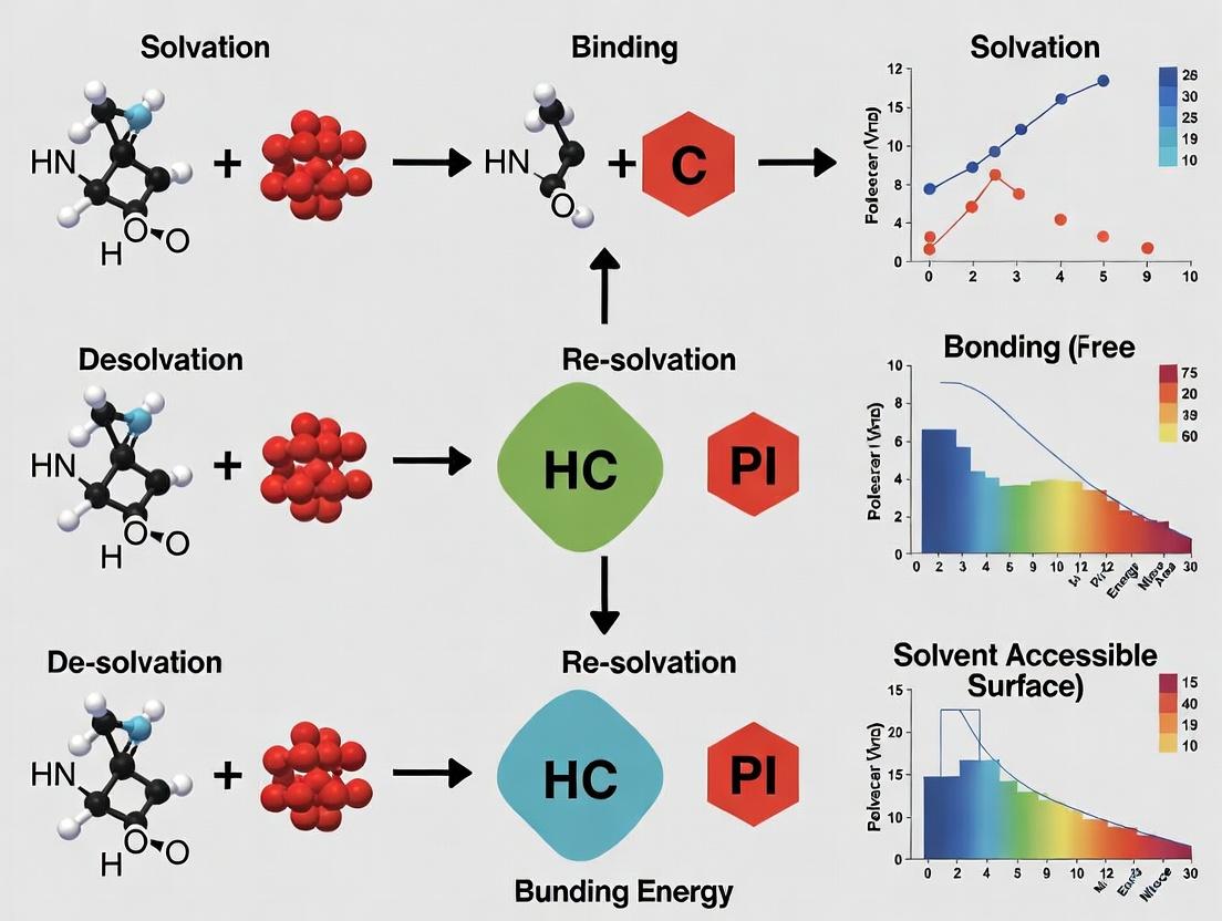
Diagram 1: Solvation & Desolvation in Binding Thermodynamics
Diagram 2: Troubleshooting Workflow for Poor Docking Scores
Diagram 3: MM/PBSA Binding Free Energy Calculation Workflow
Troubleshooting Guides & FAQs
Q1: My implicit solvent molecular dynamics (MD) simulation shows unrealistic protein collapse. What are the primary causes and solutions? A: This is often due to an overestimation of the dielectric continuum's screening effect, leading to exaggerated intramolecular charge-charge attraction. Verify and adjust the following:
- Internal Dielectric Constant (εin): The default (often εin=1-2) may be too low for the protein interior. Try increasing it to 4-10. Protocol: Run a series of short (10-20 ns) stability simulations with εin values of 2, 4, 6, and 8. Compare the radius of gyration (Rg) to a known experimental structure or an explicit solvent control.
- Salt Concentration: Implicit solvent models like Generalized Born (GB) require explicit definition of ionic strength. Use a physiologically relevant concentration (e.g., 150 mM NaCl). Protocol: In your MD input file (e.g., for AMBER or OpenMM), explicitly set the
saltconor equivalent parameter to 0.15.
Q2: When using an implicit solvent model for docking, my calculated binding energies are consistently too favorable (overly negative) compared to experimental data. How do I calibrate them? A: This typically indicates a lack of entropy or desolvation penalty terms. Implement a post-docking scoring correction.
- Protocol:
- Dock a set of 20-50 known ligands (with published binding affinities, Kd/IC50) into your target using your standard implicit solvent docking workflow.
- Record the primary docking score (e.g., GB energy, MM/GBSA ΔG).
- Perform a linear regression analysis between the computed scores and the experimental -log(Kd or IC50) (pKd/pIC50).
- Apply the resulting scaling factor and offset to all future docking scores to obtain calibrated, more predictive values.
Q3: My hybrid explicit/implicit "water cap" simulation is crashing due to water molecules evaporating from the surface. How can I stabilize it? A: This requires the application of positional restraints or a confining potential at the boundary.
- Protocol (using AMBER/NAMD):
- Define the explicit solvent region (a sphere or cylinder around the solute).
- Apply harmonic positional restraints (force constant of 1-5 kcal/mol/Ų) to all water oxygen atoms located within a 1-2 Šthick shell at the boundary of the explicit region.
- Alternatively, use a soft half-harmonic potential (a "wall" constraint) that only acts on waters attempting to leave the defined region.
Q4: How do I choose the correct implicit solvent model (e.g., GB-Neck, GB-OBC, PBSA) for my system of nucleic acids and ions? A: Nucleic acids have high charge density and specific ion interactions. Recommendations based on recent benchmarks:
- For MD Stability: Use the GB-Neck2 model, which better handles the elongated shape of DNA/RNA grooves.
- For Binding Affinity (MM/PBSA): Use the PB model over GB for final scoring, as it more accurately handles the electrostatic contributions of ions. However, for per-frame energy decomposition in MD, MM/GBSA is computationally feasible.
- Critical Step: Always include explicit counterions (e.g., Na+, K+, Mg2+) within the implicit solvent shell, as the continuum cannot fully capture specific ion binding.
Table 1: Computational Cost & Accuracy Benchmark for Solvation Models
| Solvent Model | Relative Speed (Sim. ns/day) | Typical Use Case | Relative Error in ΔGbind (kcal/mol) | Key Limitation |
|---|---|---|---|---|
| Explicit (TIP3P) | 1x (Baseline) | High-accuracy MD, ion binding | ~1.0 (Baseline) | Extreme computational cost |
| Implicit (GB-OBC2) | 50-100x | High-throughput docking, MD folding | 2.0 - 4.0 | Poor charge screening, no explicit H-bonds |
| Implicit (GB-Neck2) | 40-80x | Nucleic acid MD, protein stability | 1.5 - 3.5 | Better for elongated shapes, higher cost |
| Hybrid (Water Cap) | 10-20x | Membrane protein surface loops | 1.5 - 2.5 | Boundary artifacts |
Table 2: Recommended Implicit Solvent Parameters for Common Systems
| System Type | Internal Dielectric (εin) | External Dielectric (εout) | Salt Conc. (M) | Recommended Software Implementation |
|---|---|---|---|---|
| Globular Protein (Ligand Docking) | 2 - 4 | 78.5 | 0.15 | AutoDock-GPU, AutoDock Vina, Schrödinger Glide |
| Protein Folding/Unfolding MD | 4 - 10 | 78.5 | 0.15 | AMBER (igb=8), OpenMM (GB-Neck2) |
| Protein-Nucleic Acid Complex | 4 - 6 | 78.5 | 0.15 - 0.20 | AMBER (igb=8, mbondi3 radii) |
| Small Molecule Solvation | 1 | 78.5 | 0.00 | Gaussian (SMD), AMSOL |
Experimental Protocols
Protocol 1: Validation of Implicit Solvent Parameters via Radius of Gyration (Rg) Objective: To calibrate εin by comparing protein compactness in implicit solvent to an explicit solvent reference.
- System Preparation: Obtain a crystal structure of a well-folded protein (e.g., Lysozyme, PDB: 1AKI). Remove ligands and solvent. Add missing hydrogen atoms using
pdb4amberorLEaP. - Explicit Control Simulation: Solvate the protein in a TIP3P water box with 10 Å padding. Add 0.15 M NaCl. Minimize, heat, equilibrate (NPT, 310K, 1 bar). Run a 50 ns production MD simulation (AMBER/NAMD/GROMACS).
- Implicit Test Simulations: Prepare the same protein structure. Create 4 separate parameter sets with εin = 2, 4, 6, and 8 (εout=78.5, saltcon=0.15). Run four separate 50 ns production MD simulations in implicit solvent (no periodic boundary conditions needed).
- Analysis: For all 5 trajectories, calculate the Rg over time using
cpptrajorgmx gyrate. Compute the average and standard deviation over the last 40 ns. The implicit solvent condition with an average Rg closest to the explicit solvent control is selected for future studies.
Protocol 2: MM/PBSA Binding Free Energy Calculation Workflow Objective: To estimate the binding free energy for a protein-ligand complex from an explicit solvent MD trajectory.
- Explicit Solvent MD: Run a standard, well-equilibrated explicit solvent MD simulation of the protein-ligand complex.
- Trajectory Sampling: Extract 100-500 evenly spaced snapshots from the stable production phase.
- Energy Calculations (Per Snapshot):
- Strip waters and ions from each snapshot.
- Calculate the vacuum molecular mechanics energy (EMM) for the complex, receptor, and ligand.
- Calculate the Poisson-Boltzmann (PB) solvation energy (ΔGPB) and nonpolar solvation energy (ΔGSA, from SASA) for each species.
- Free Energy Averaging: Use the MM/PBSA formula for each snapshot
i: ΔGbind,i = Gcomplex,i - Greceptor,i - Gligand,i where G = EMM + ΔGPB + ΔGSA - TS (entropy often omitted). The final reported ΔGbind is the average over all snapshots, with standard error.
Diagrams
Decision Workflow for Solvent Model Selection
Solvent Model Selection Logic Tree
The Scientist's Toolkit: Research Reagent Solutions
| Item/Software | Function in Solvation Modeling | Example/Provider |
|---|---|---|
| AMBER | Molecular dynamics suite with advanced GB (OBC, Neck) and PB solvers for implicit solvent simulations. | ambermd.org |
| OpenMM | GPU-accelerated toolkit supporting multiple implicit solvent models (GBSA, OBC, Neck2) for fast sampling. | openmm.org |
| AutoDock Vina | Widely-used docking program with a fast, built-in implicit solvent scoring function for high-throughput screening. | vina.scripps.edu |
| GMX | GROMACS tool for PBSA calculations (g_mmpbsa) on explicit solvent trajectories. |
gromacs.org |
| PDB2PQR | Prepares structures for PB calculations by adding hydrogens, assigning charges (AMBER/CHARMM), and setting radii. | pdb2pqr.org |
| APBS | Solves the Poisson-Boltzmann equation for electrostatic potentials and solvation energies in complex biomolecules. | poissonboltzmann.org |
| MOLARIS | Specialized for simulations with generalized Born and other implicit solvent models, emphasizing electrostatic effects. | Enzymix.com |
| NAMD | High-performance MD simulator capable of hybrid explicit/implicit (GBIS) solvent simulations for large systems. | ks.uiuc.edu |
AMBER Parameter Sets (e.g., leaprc.protein.ff19SB) |
Provide the force field parameters (bonded & nonbonded) essential for accurate energy calculations in any solvent model. | ambermd.org |
Ligand Parameterization Tools (e.g., antechamber, CGenFF) |
Generate force field parameters for small molecule inhibitors/drugs, a prerequisite for consistent implicit/explicit simulation. | ambermd.org, cgenff.umaryland.edu |
Troubleshooting & FAQ Hub
Q1: My binding affinity calculations with an implicit solvent model show poor correlation with experimental data. What could be the cause? A: This is a common issue. Primary culprits include: 1) An inappropriate choice of the dielectric constant (ε). A constant value for the solute (e.g., ε=1-4) and solvent (e.g., ε=80 for water) is typical, but this oversimplifies local heterogeneity. 2) Inadequate treatment of the non-electrostatic component of the solvation free energy (cavity formation and dispersion interactions). 3) The Potential of Mean Force (PMF) derived from your model may not accurately capture specific, directional interactions like hydrogen bonds. Troubleshoot by comparing results using different ε values for the solute (e.g., 1, 2, 4) and verifying the parameterization of your non-polar solvation term.
Q2: How do I decide between using a distance-dependent dielectric function (ε=r) and a constant dielectric continuum model? A: A distance-dependent dielectric (e.g., ε=r) is an older, crude approximation used to mimic solvent screening in vacuo, largely superseded by more physical models. It should be avoided for quantitative analysis of solvation. The constant dielectric continuum model (e.g., Poisson-Boltzmann or Generalized Born) is fundamentally more sound for representing bulk solvent effects. Use a constant dielectric model for any serious docking or binding free energy study.
Q3: What is the "dielectric boundary," and why does its definition cause numerical instability in my Poisson-Boltzmann calculations? A: The dielectric boundary defines where the low-dielectric solute (εin) transitions to the high-dielectric solvent (εout). It is typically the molecular surface. Instability arises from: 1) Grid Discretization: If the grid spacing is too coarse, the boundary is poorly resolved. 2) Surface Definition: Sharp corners or narrow cavities in the molecular surface can lead to large field fluctuations. Solution: Refine your finite-difference grid (use a spacing of 0.5 Å or finer), try a smoother surface definition (like a solvent-accessible surface with a larger probe), or switch to a Generalized Born model, which approximates the Poisson result but is less sensitive to boundary details.
Q4: How does the Potential of Mean Force (PMF) relate to the free energy I obtain from my implicit solvent docking score? A: Your docking score is an approximation of the PMF. In implicit solvent theory, the solvent-averaged interactions are embedded into the effective potential (the PMF) used to simulate the solute. Therefore, a well-parameterized docking scoring function should represent the PMF for the solute degrees of freedom. A large discrepancy between docking ranks and experimental binding affinities suggests the scoring function's implicit PMF is flawed.
Q5: Can implicit solvent models capture specific binding water molecules, which are critical for my protein-ligand complex? A: Standard continuum models cannot. They treat water as a uniform dielectric medium, annihilating all structural details. This is a major limitation. If crystallographic data shows conserved, mediating water molecules, you must treat them as explicit part of the solute. Advanced hybrid approaches ("explicit implicit") exist, where key waters are modeled explicitly, and the bulk is treated as a continuum.
Table 1: Common Dielectric Constant Values Used in Implicit Solvent Models
| Region / Material | Typical Dielectric Constant (ε) | Notes |
|---|---|---|
| Protein Interior | 2 - 4 | Lower values (2-4) for hydrophobic cores; higher (4-20) for polar regions. |
| Lipid Bilayer | 2 - 3 | Highly hydrophobic environment. |
| Water (Bulk) | 78.4 - 80 | At 25°C. Most common value is 80. |
| DNA/RNA Sugar-Phosphate Backbone | ~10-20 | Depends on ionic strength and model. |
| Distance-Dependent Approximation | ε = r (in Å) | Historical use; not recommended for accurate work. |
Table 2: Comparison of Implicit Solvent Method Characteristics
| Method | Electrostatic Treatment | Speed | Handling of Solvent Boundary | Common Implementation |
|---|---|---|---|---|
| Poisson-Boltzmann (PB) | Solves PB equation numerically. | Slow | Sensitive to definition and grid. | APBS, DelPhi, Amber |
| Generalized Born (GB) | Approximates PB result analytically. | Fast | More robust, less accurate. | Amber, CHARMM, OpenMM |
| COSMO | Conductor-like screening model. | Fast | Treats solvent as ideal conductor. | TURBOMOLE, ORCA |
Experimental Protocol: Validating an Implicit Solvent Model for Docking
Objective: To assess the performance of a chosen implicit solvent model within a docking workflow by correlating computed scores with experimentally determined binding affinities (pKi or pIC50).
Materials:
- A curated dataset of 50-100 protein-ligand complexes with known high-resolution structures (from PDB) and reliable binding affinity data.
- Docking software (e.g., AutoDock Vina, GOLD, Schrodinger Glide) configured to use the implicit solvent model under test.
- Molecular visualization software (e.g., PyMOL, Chimera).
- Scripting environment (Python/R) for statistical analysis.
Procedure:
- Dataset Preparation: Prepare protein structures (remove waters except critical ones, add hydrogens, assign partial charges) and ligand structures (generate 3D conformers, assign charges) in formats compatible with your docking software.
- Grid/Search Space Definition: For each complex, define the docking search box centered on the cognate ligand's position.
- Docking Run: Dock each ligand to its target protein using the standard scoring function with and without (vacuum control) the implicit solvent model. Use consistent, extensive search parameters.
- Score Extraction: Record the best (lowest) docking score for each complex from both runs.
- Data Analysis: Calculate the Pearson (R) and Spearman (ρ) correlation coefficients between the docking scores and the negative log of the experimental binding affinity (-log(Ki/IC50)).
- Validation: The model yielding the higher correlation coefficient (R and ρ) and lower root-mean-square error (RMSE) provides a better implicit representation of solvation for your system class.
Visualizations
Title: From Explicit Solvent to Implicit Continuum and PMF
Title: Implicit Solvent Model Validation Workflow
The Scientist's Toolkit: Essential Reagents & Materials
Table 3: Key Research Reagent Solutions for Implicit Solvent Studies
| Item | Function in Context |
|---|---|
| Protein Data Bank (PDB) Structures | Source of high-resolution 3D coordinates for the solute (protein/ligand complex). Essential for defining the dielectric boundary. |
| Curated Binding Affinity Databases (e.g., PDBbind, BindingDB) | Provides experimental benchmark data (Ki, IC50) for validating and parameterizing the implicit solvent PMF. |
| Molecular Dynamics/Simulation Software (e.g., AMBER, GROMACS, CHARMM) | Often used to parameterize or validate implicit solvent models by comparing to explicit solvent simulations (the "ground truth"). |
| Continuum Electrostatics Solvers (e.g., APBS for PB, GB models in Amber) | The core computational engines that calculate electrostatic solvation free energies for a given dielectric model. |
| Docking Software with Implicit Solvent Options (e.g., AutoDock Vina, Glide, Gold) | Provides the integrated application environment where the implicit solvent PMF is used as part of the scoring function. |
| Scripting Tools (Python with NumPy/SciPy, R) | Critical for automating workflows, processing docking outputs, and performing statistical correlation analyses. |
Technical Support & Troubleshooting Center
This support center addresses common computational and conceptual issues encountered when working with solvation free energy components in the context of implicit solvent models for molecular docking research.
Frequently Asked Questions (FAQs)
Q1: During MM/PBSA calculations for docking post-processing, my polar solvation energy (ΔGpolar) values are anomalously high and positive, making favorable ligands appear unstable. What could be the cause? A: This is often due to incorrect interior dielectric constant (εin) assignment. The default εin=1 is for vacuum; for protein interiors, a value between 2-4 is more realistic. Solution: Re-run the Poisson-Boltzmann calculation with an adjusted ε_in (e.g., 2 or 4). Also, verify your atomic radii set (e.g., Bondi, PARSE, mbondi2) matches the parameter set of your force field.
Q2: When comparing implicit solvent models (GB vs. PB), the non-polar contribution varies significantly. Which model is more reliable for docking poses? A: The non-polar term is typically decomposed into cavity dispersion (cavity) and van der Waals (dispersion) components. Poisson-Boltzmann (PB) models often use a surface area (SA) term (γSASA + b), while Generalized Born (GB) models may incorporate a more empirical approach. For docking, consistency is key. *Recommendation: Use the same model and parameters (γ and b) for all comparative analyses. The table below summarizes common parameter sets.
Q3: My cavity formation energy, calculated via the Surface Area (SA) term, seems insensitive to small ligand changes. Is this expected? A: Yes, to an extent. The cavity term (γ*SASA) is linearly proportional to the solvent-accessible surface area. Small conformational changes in a ligand of fixed chemical composition may yield small SASA changes. For high-precision work, consider models that include a curvature correction or a volume-based term. Ensure your SASA calculation uses a consistent probe radius (typically 1.4 Å for water).
Q4: How do I decide between a polar and a non-polar implicit solvent model for a virtual screening campaign? A: This depends on your target system. Use the decision guide below:
Title: Solvent Model Selection for Virtual Screening
Table 1: Common Parameter Sets for Non-Polar Solvation Energy (ΔGnonpolar = γ * SASA + b)
| Parameter Set | γ (kcal/mol/Ų) | b (kcal/mol) | Best Used With | Notes |
|---|---|---|---|---|
| PARSE | 0.00542 | 0.92 | PB/SA, Folding Studies | Derived from protein folding data. |
| LCPO | 0.005 | 0.00 | GB/SA, MD Simulations | Default in many MD packages. Efficient SASA approximation. |
| Shouldberg | 0.0072 | 0.00 | Small Molecule Solvation | Optimized for small organic molecule transfer energies. |
Table 2: Comparison of Implicit Solvent Model Components
| Model | Polar Term Method | Non-Polar/Cavity Term | Computational Cost | Typical Use Case in Docking |
|---|---|---|---|---|
| Poisson-Boltzmann (PB) | Solves PDE for electrostatic potential. | γ*SASA + b | High | Final scoring, MM/PBSA. |
| Generalized Born (GB) | Approximates PB using pairwise screening. | γ*SASA (often) | Medium | Rescoring, MD pre-processing. |
| SASA-Only | Neglected or constant. | γ*SASA + b | Very Low | Initial hydrophobic filter. |
Experimental & Computational Protocols
Protocol 1: Calculating Solvation Free Energy Components Using MM/PBSA Objective: To decompose the solvation free energy (ΔGsolv) of a docked protein-ligand complex into polar and non-polar components.
- Input Preparation: Generate optimized docked poses. Prepare topology files for the complex, receptor, and ligand using a compatible force field (e.g., AMBER ff19SB, GAFF2).
- Trajectory Generation: Perform a short, implicit solvent minimization and MD simulation (GB model) on the complex to generate an ensemble (e.g., 100 snapshots).
- Energy Calculation: For each snapshot, calculate:
- ΔGpolar: Using the
pbsamodule to solve the PB equation. Key parameters:indi=2.0, exdi=80.0, istrng=0.15. - ΔGnonpolar: Calculate SASA (e.g., via
molsurf) and apply the LCPO parameters: γ=0.005 kcal/mol/Ų, b=0.0.
- ΔGpolar: Using the
- Averaging & Analysis: Average ΔGpolar and ΔGnonpolar over all snapshots. ΔGsolv = <ΔGpolar> + <ΔGnonpolar>.
Protocol 2: Benchmarking Cavity Term Parameters for a Congeneric Series Objective: To empirically test which (γ, b) parameter set best predicts experimental binding affinities for a series of similar ligands.
- Data Curation: Obtain a set of 10-20 ligands with known experimental ΔGbind against the same target. Prepare their docked poses.
- Single-Point Calculation: For each ligand pose, calculate the cavity formation energy using 3-4 different parameter sets (see Table 1). Use a fixed, minimized receptor structure.
- Correlation Analysis: Plot calculated cavity energy vs. experimental ΔGbind for each parameter set. Perform linear regression.
- Selection: Choose the parameter set yielding the highest correlation (R²) for your specific system class.
The Scientist's Toolkit: Research Reagent Solutions
Table 3: Essential Software & Computational Tools
| Item | Function & Relevance | Example/Version |
|---|---|---|
| Molecular Dynamics Engine | Samples conformational space; calculates energy terms. | AMBER, NAMD, GROMACS |
| Continuum Solvent Solver | Computes polar (PB/GB) solvation energies. | APBS, PBSA in AMBER, sander |
| SASA Calculator | Computes solvent-accessible surface area for cavity term. | molsurf (AMBER), FreeSASA, NACCESS |
| Force Field Parameterization | Provides charges and vdW radii for polar/non-polar terms. | antechamber (for GAFF), tleap |
| Scripting Framework | Automates analysis and data pipelining. | Python (MDAnalysis, pandas), Bash |
| Visualization Suite | Inspects poses, surfaces, and electrostatic potentials. | PyMOL, VMD, ChimeraX |
Title: MM/PBSA Solvation Component Workflow
Implementing Implicit Solvation: From Theory to Docking Workflow Integration
Troubleshooting Guides & FAQs
FAQ 1: My docking scores are unrealistically favorable when using a GB model. What could be wrong? Answer: This is often due to incorrect assignment of atomic radii or internal dielectric constant.
- Check 1: Ensure you are using a consistent set of optimized radii (e.g., Bondi, mbondi2, mbondi3) for both your protein and ligand. Mismatched sets cause errors in the Born energy calculation.
- Check 2: The internal dielectric constant (
intdiel) is crucial. For docking rigid proteins, a value of 2-4 is typical. A value of 1 (vacuum) can overestimate electrostatic interactions. For flexible docking or to account for protein reorganization, a value of 4-20 may be more appropriate. Test a range of values. - Protocol: Run a control calculation on a system with known binding affinity. Systematically vary
intdiel(e.g., 1, 2, 4, 8) and the radii set, comparing the computed solvation energy to a reference Poisson-Boltzmann (PB) solution or experimental data.
FAQ 2: When comparing PCM and GB results for ligand solvation free energy, I get large discrepancies. Which should I trust? Answer: Discrepancies often stem from the treatment of the solute cavity and non-electrostatic terms.
- Check 1: Verify that the molecular surface (PCM) vs. the pairwise atomic sphere model (GB) is the primary cause. PCM is generally more accurate but computationally heavier.
- Check 2: Ensure non-electrostatic terms (cavitation, dispersion, repulsion) are included consistently. Some GB implementations only compute the electrostatic term, while PCM often includes all terms. Missing terms in GB can cause significant errors.
- Protocol:
- Single-Point Energy: Compute the solvation free energy (
ΔGsolv) for a small molecule in water using both models with the same geometry and high-level theory (e.g., DFT). - Decompose Energy: Output the electrostatic and non-electrostatic components separately.
- Compare: Use a table to compare components against experimental or high-level benchmark data (see Table 1).
- Single-Point Energy: Compute the solvation free energy (
FAQ 3: My Poisson-Boltzmann (PB) calculation fails or produces NaN results for a large protein-ligand complex. Answer: This is typically a grid-related issue.
- Check 1: The finite-difference grid may be too coarse or not properly centered. Ensure the grid spacing is ≤ 0.5 Å and the complex is centered with at least 10 Å of padding on all sides.
- Check 2: Check for "buried" charged atoms. If an atom with a high partial charge is deep inside the molecule, it can cause numerical instability. Consider using a finer grid locally or switching to a GB model for initial scans.
- Protocol:
- Increase grid points (e.g., from 65³ to 97³ or 129³).
- Set focus (sequential focusing) to iteratively solve from a coarse to a fine grid.
- Use an adaptive (mg-auto) grid if your software supports it.
FAQ 4: How do I choose between a SASA-based and an electrostatics-based (GB/PB) model for virtual screening? Answer: The choice depends on the dominant binding forces of your target system.
- Use SASA-based (e.g., Linear Combination of Pairwise Overlap, LCPO): For initial, ultra-high-throughput screening where hydrophobic effects are believed to dominate, or for ranking congeneric series with similar electrostatic profiles. It's fast but neglects explicit electrostatics.
- Use GB or PB: For systems where electrostatic steering, salt bridges, or desolvation penalties for charged groups are critical (e.g., kinase ATP-binding sites, ionic interactions). Use PB for final, accurate scoring and GB for intermediate throughput with better physics than SASA.
- Protocol: Perform a retrospective validation on known actives/decoys. Rank compounds using both a SASA term (like AGBNP) and a full GB model (like OBC/GBSA). Compare the enrichment factors (EF1%) and ROC curves to decide which model performs better for your specific target.
Table 1: Comparison of Implicit Solvent Model Characteristics
| Model Family | Key Strength | Key Limitation | Typical Relative Speed (vs. Explicit) | Common Use Case in Docking |
|---|---|---|---|---|
| Poisson-Boltzmann (PB) | High accuracy for electrostatics; rigorous. | Slow; grid dependencies; numerical instability. | 10² - 10³ | Final binding affinity refinement; small molecule ∆Gsolv calculation. |
| Generalized Born (GB) | Good accuracy/speed balance; analytic. | Approximates dielectric boundary; radii-dependent. | 10⁴ - 10⁵ | Post-docking scoring (MM/GBSA); molecular dynamics. |
| PCM/COSMO | Quantum chemistry compatible; good for diverse solvents. | Very slow; QM-level calculations required. | 10² - 10³ (QM level) | QM/MM studies; ligand parameterization. |
| SASA-based | Extremely fast; simple. | No explicit electrostatics; empirical. | 10⁶ - 10⁷ | First-pass virtual screening; hydrophobic packing scoring. |
Table 2: Common Parameterization Issues & Fixes
| Symptom | Likely Cause | Recommended Troubleshooting Action |
|---|---|---|
| Overly favorable scores for charged ligands. | Internal dielectric constant too low. | Increase intdiel from 1 to 2-4 for rigid receptor docking. |
| Poor correlation with experiment for polar compounds. | Missing or incorrect non-polar term. | Add/calibrate a SASA-based term (γ*SASA + b). |
| High sensitivity to minor conformational changes. | GB model with sharp surface definition. | Switch to a smoother GB model (e.g., GBNSR6 vs. OBC) or use PB. |
| ∆Gsolv errors > 5 kcal/mol for anions. | Incorrect atomic radii for elements. | Use a specifically optimized radii set (e.g., mbondi3 for OPLS-AA). |
Experimental Protocols
Protocol 1: MM/GBSA Binding Free Energy Calculation (Post-Docking Refinement) Purpose: To re-score docking poses with a more physically rigorous implicit solvation model. Method:
- Input: Generate an ensemble of protein-ligand complexes from molecular docking (e.g., 50-100 poses per ligand).
- Minimization: Perform limited minimization (e.g., 500 steps steepest descent) on each complex in vacuo to remove severe clashes, keeping the protein backbone restrained.
- Single-Point Energy Calculation: For each minimized structure, calculate the gas-phase MM energy (EMM), the GB solvation energy (GGB), and the SASA-based non-polar energy (GSA).
- Calculation: Compute the binding free energy estimate: ΔGbind ≈ ΔEMM + ΔGGB + ΔGSA - TΔS (often entropy is omitted for ranking).
- Averaging: Average the ΔGbind values over the ensemble of poses for each ligand.
- Validation: Rank ligands by average ΔGbind and compute correlation with experimental Ki/IC50 values.
Protocol 2: Benchmarking Solvation Models for Ligand Parameterization Purpose: To select the best implicit solvent model for calculating ligand solvation free energies for force field development. Method:
- Dataset: Select a benchmark set of 50-200 diverse organic molecules with experimental hydration free energies (e.g., MNSOL or FreeSolv database).
- Geometry Optimization: Optimize each molecule's geometry at the DFT/B3LYP/6-31G* level in vacuum.
- Single-Point Solvation Energy: For each optimized structure, perform a single-point energy calculation in:
- Vacuum.
- Implicit solvent (Water) using the target models: PCM, SMD, GB (multiple radii sets), and a reference PB model.
- Compute ΔGsolv: ΔGsolv = E(solvent) - E(vacuum) + G(non-electrostatic).
- Statistical Analysis: Calculate the Mean Absolute Error (MAE), Root Mean Square Error (RMSE), and linear correlation coefficient (R²) for each model against experimental data.
- Selection: Choose the model with the best compromise between accuracy (low MAE, high R²) and computational cost for your intended application.
Visualization
Diagram 1: Implicit Solvent Model Selection Workflow
Diagram 2: MM/GBSA Post-Docking Refinement Protocol
The Scientist's Toolkit: Research Reagent Solutions
Table 3: Essential Software & Parameter Sets for Implicit Solvent Studies
| Item Name | Function/Brief Explanation | Typical Application |
|---|---|---|
| APBS | Software for solving the Poisson-Boltzmann equation numerically. | Calculating electrostatic potentials and solvation energies for biomolecules. |
| GB models (OBC, GBNSR6) | Specific Generalized Born implementations offering speed/accuracy trade-offs. | Solvation energy calculations in MD packages (AMBER, GROMACS) and MM/GBSA. |
| Gaussian with PCM/SMD | Quantum chemistry software with integrated implicit solvent models. | Calculating accurate solvation energies for small molecules and ligands. |
| Optimized Radii Sets (mbondi2, mbondi3) | Parameter sets defining atomic radii for GB/PB calculations. | Ensuring consistent and accurate dielectric boundary definition; critical for results. |
| AGBNP/AGBNP2 | Analytic generalized Born model with non-polar parameterization. | Implicit solvent for MD and scoring in docking software like Vina. |
| MSMS | Software for molecular surface triangulation. | Generating the solute-solvent boundary for PB and some GB models. |
Integrating Implicit Solvation into Docking Scoring Functions (e.g., MM/PBSA, MM/GBSA)
Technical Support Center: Troubleshooting Guides & FAQs
This support center is framed within the thesis context of advancing docking research by addressing the critical role of solvation effects through implicit solvent models like MM/PBSA and MM/GBSA. The following FAQs address common experimental pitfalls.
Frequently Asked Questions (FAQs)
Q1: Why do I get excessively favorable (overly negative) binding free energies when running MM/PBSA calculations on my docked protein-ligand complex? A: This is often due to inadequate sampling. A single, static docked pose does not represent the conformational ensemble of the binding event. The implicit solvation energy is highly sensitive to small atomic displacements. Solution: Perform molecular dynamics (MD) simulation to generate an ensemble of snapshots from the trajectory for MM/PBSA or MM/GBSA analysis, rather than using a single minimized docked structure.
Q2: My MM/GBSA results show high variance between snapshots. Is this normal, and how can I improve consistency? A: Some variance is expected, but high fluctuations often indicate an unstable trajectory or insufficient equilibration. Solution: 1) Extend the equilibration phase of your MD simulation. 2) Ensure your system is properly neutralized and ion concentration is physiologically relevant. 3) Use a longer production simulation to improve sampling. Calculate the moving average of the binding free energy to assess convergence.
Q3: What are the key differences between PBSA and GBSA models in scoring, and how do I choose? A: The core difference lies in how the electrostatic solvation free energy is calculated. PBSA solves the Poisson-Boltzmann equation numerically on a grid, which is more accurate but computationally expensive. GBSA uses the Generalized Born approximation, which is faster but less accurate, particularly for systems with high charge density or deep binding pockets. Solution: Use PB for final, high-accuracy scoring on select complexes. Use GB for high-throughput screening or initial ranking due to its speed.
Q4: How should I handle protonation states of titratable residues and the ligand before MM/PBSA/GBSA calculation?
A: Incorrect protonation states are a major source of error. Solution: Use a tool like PDB2PQR, PROPKA, or H++ to determine the likely protonation state of key residues (e.g., His, Asp, Glu) at your target pH (typically 7.4) before docking and MD set-up. For the ligand, use chemical knowledge or perform a preliminary quantum mechanics (QM) optimization.
Q5: Why does the binding entropy term (often from NMA) sometimes worsen the correlation with experimental data? A: The normal mode analysis (NMA) for entropy is calculated in the gas phase and is highly sensitive to the local minima of the minimized structure. It can introduce noise, especially for flexible systems. Solution: Many studies use the enthalpy-only term (MM/PB(GB)SA) for ranking. Consider using the more advanced quasi-harmonic analysis on the MD trajectory for entropy, though it is more costly. Evaluate with and without the entropy term for your specific system.
Detailed Experimental Protocol: MM/PBSA from a Docked Pose
This protocol outlines the steps to calculate binding free energy using MM/PBSA, starting from a docked protein-ligand complex.
System Preparation:
- Input: Docked complex PDB file.
- Process: Use a tool like
LEaP(AmberTools) orpdb4amberto add missing hydrogen atoms. Assign correct protonation states (see FAQ Q4). Strip away crystallographic water molecules unless one is known to be crucial for binding. - Output: A fully protonated PDB file ready for force field assignment.
Parameter and Topology Generation:
- Assign a force field (e.g., ff19SB for protein, GAFF2 for ligand) using
tleap(Amber) or similar. The ligand's partial charges must be derived, typically via antechamber using the AM1-BCC method. - Generate the topology and coordinate files for the complex, the receptor alone, and the ligand alone.
- Assign a force field (e.g., ff19SB for protein, GAFF2 for ligand) using
System Solvation and Neutralization:
- Solvate the complex in an explicit water box (e.g., TIP3P) with a buffer distance of at least 10 Å.
- Add counterions to neutralize the system's net charge. For physiological realism, add additional salt (e.g., 150 mM NaCl).
Molecular Dynamics Simulation:
- Minimization: Perform 2-stage minimization: 1) Solvent only, holding solute restrained. 2) Full system.
- Heating: Gradually heat the system from 0 K to 300 K over 50-100 ps under NVT ensemble with weak restraints on solute.
- Equilibration: Run 1-5 ns of NPT equilibration at 300 K and 1 bar to density the system. Release restraints gradually.
- Production: Run an unrestrained MD simulation. The length depends on system size and flexibility; 20-100 ns is common. Save snapshots every 10-100 ps for later analysis.
MM/PBSA Calculation:
- Extract snapshots from the production trajectory at regular intervals (e.g., every 100 ps).
- Use the
MMPBSA.py(Amber) orgmx_MMPBSA(GROMACS) module to calculate energies for each snapshot. - The script decomposes the trajectory into receptor (R) and ligand (L) components and calculates:
- Gas-phase MM energy (EMM = Ebonded + EvdW + Eele).
- Polar solvation energy (ΔGPB or ΔGGB) by solving PB/GB.
- Non-polar solvation energy (ΔGSA) from the solvent-accessible surface area (SASA).
- The final binding free energy for snapshot i is: ΔGbind,i = Gcomplex,i - Greceptor,i - Gligand,i, where G = EMM + ΔGsolv - TS. The average ΔGbind is reported.
Data Presentation: Comparison of Implicit Solvation Models
Table 1: Key Characteristics and Performance Metrics of Implicit Solvation Methods in Docking Scoring.
| Method | Computational Speed | Key Strengths | Key Limitations | Typical Use Case in Docking |
|---|---|---|---|---|
| MM/PBSA | Slow (Minutes per snapshot) | High accuracy for electrostatic interactions; rigorous treatment of dielectric boundaries. | Sensitive to atomic radii and internal dielectric constant; slow for high-throughput. | Post-docking refinement and ranking of top candidate complexes. |
| MM/GBSA | Moderate (Seconds per snapshot) | Good balance of speed and accuracy; suitable for larger systems. | Less accurate for highly charged systems, anions, and deep pockets. | Virtual screening, ranking hundreds to thousands of docked poses. |
| GB-SW (Surface Generalized Born) | Fast (Sub-second per pose) | Very fast; often integrated directly into docking scoring functions. | Simplified model; can be less accurate for detailed binding energy prediction. | Real-time scoring during molecular docking simulations. |
Table 2: Impact of Protocol Choices on MM/PBSA/GBSA Results (Hypothetical Benchmark Data).
| Protocol Variable | Default/Common Choice | Alternative | Observed Effect on ΔGbind (vs. Experiment) | Recommendation |
|---|---|---|---|---|
| Dielectric Constant (Internal) | 1 (protein), 1 (ligand) | 2-4 (protein) | Higher dielectric reduces electrostatic penalty, often improving correlation for polar binding sites. | Test ε=2-4 for protein if binding site is solvent-exposed. |
| Ion Concentration | 0.15 M NaCl | 0 M (no salt) | Can significantly shift ΔGbind for charged ligands by ±2-5 kcal/mol. | Always include physiological salt concentration. |
| Sampling (Snapshots) | Single minimized pose | 1000 from MD | Reduces noise and false positives; improves rank correlation (R² from ~0.3 to ~0.6 in benchmarks). | Always use MD-based ensemble, not a single pose. |
| Entropy Estimation | Not included (ΔH only) | NMA | Adds substantial noise (±3-10 kcal/mol); often worsens ranking for flexible systems. | Omit for initial ranking; include only for final, well-converged systems. |
Visualizations
Workflow for MM/PBSA Calculation from a Docked Pose
Energy Decomposition in MM/PBSA/GBSA
The Scientist's Toolkit: Research Reagent Solutions
Table 3: Essential Software and Tools for Implicit Solvation in Docking.
| Item Name | Category | Function/Brief Explanation |
|---|---|---|
AmberTools (esp. MMPBSA.py) |
Software Suite | The standard suite for running MM/PBSA and MM/GBSA calculations, including topology building and trajectory analysis. |
| gmx_MMPBSA | Software Tool | Integrates MM/PBSA/GBSA functionality with the GROMACS MD engine, a popular alternative to Amber. |
| AutoDock Vina with GB | Docking Engine | A widely used docking program that can incorporate a fast GB implicit solvation model directly into its scoring function. |
| OpenMM | MD Library | A high-performance toolkit for MD simulation that can be scripted to prepare systems for subsequent MM/PBSA analysis. |
| GAFF2 (Generalized Amber Force Field 2) | Force Field | Provides parameters for small organic molecules (ligands), essential for accurate energy calculation. |
| AM1-BCC | Charge Method | A fast and reasonably accurate method for deriving partial atomic charges for ligands for use with GAFF2. |
| PDB2PQR / PROPKA | Pre-processing Tool | Prepares PDB files by adding hydrogens and assigning protonation states of residues based on pKa prediction. |
| VMD / PyMOL | Visualization | Critical for inspecting docked poses, MD trajectories, and visualizing binding interactions pre- and post-analysis. |
Technical Support Center
Troubleshooting Guides
Issue 1: APBS Fails to Calculate Potentials for Large PQR Files
- Problem: Job terminates with memory allocation errors or segmentation faults.
- Diagnosis: The system's grid dimensions are too large, exceeding available RAM. This is common for large complexes or fine grid spacing.
- Solution: Use the
--splitoption inpqr2gridto decompose the calculation. Alternatively, coarsen the grid spacing (dimekeyword in APBS input file) or reduce the computational box size (cglen/fglen). Always check the estimated memory requirement from APBS's initial output.
Issue 2: DISOLV (or Similar Poisson-Boltzmann Solver) Returns Unphysical Binding Energies
- Problem: Calculated ΔΔG values are orders of magnitude too high or low.
- Diagnosis: Incorrect assignment of atomic radii or internal dielectric constant (ε_in).
- Solution: Ensure consistency between the force field used for PQR generation (e.g., AMBER, CHARMM) and the corresponding parameter set in the solver. For protein-ligand docking, ε_in is typically between 1-4. Validate with a known benchmark system.
Issue 3: Integrated Solvation Model in Docking Suite (e.g., AutoDock-GPU's Solvation Term) is Non-Adjustable
- Problem: The user cannot modify solvation parameters within the GUI or standard docking parameters file, limiting model flexibility.
- Diagnosis: The solvation model is hard-coded as a simplified term (e.g., a weighted surface area term) for computational speed.
- Solution: Consult the software's advanced documentation. Some suites allow modification via source code recompilation or a secondary configuration file (e.g.,
AD4_parameters.datin AutoDock4). If not, consider post-scoring docking poses with a stand-alone solver for more accurate solvation energy assessment.
Issue 4: Inconsistency Between Solvation Energies from Stand-Alone vs. Integrated Solvers
- Problem: For the same ligand pose, solvation energies differ significantly between an APBS calculation and the docking suite's internal score.
- Diagnosis: Fundamental differences in the implicit solvent model (e.g., full Poisson-Boltzmann vs. Generalized Born vs. simple SASA), and different nonpolar solvation models.
- Solution: This is often expected. Use the Experimental Protocol for Benchmarking Solvation Models below to establish baseline correlations for your specific system class. Choose the tool whose relative rankings best match experimental binding data.
Frequently Asked Questions (FAQs)
Q1: When should I use a stand-alone solver like APBS over my docking software's built-in solvation model? A1: Use APBS (or similar) for post-processing and rigorous binding energy analysis (MM/PBSA, MM/GBSA) after docking. Use the integrated model for high-throughput screening where speed is critical. Stand-alone solvers offer greater accuracy and control over physical parameters (dielectric constants, ion strength, nonpolar model).
Q2: What are the key computational trade-offs between accuracy and speed? A2: See the quantitative comparison in Table 1.
Table 1: Performance & Accuracy Comparison of Solvent Models
| Model / Implementation | Typical Speed (poses/sec)* | Accuracy Relative to Exp. ΔG | Key Tunable Parameters |
|---|---|---|---|
| APBS (PBE) | 1 - 10 | High | εin, εout, ion conc., grid fineness, nonpolar model |
| DISOLV (GB) | 100 - 1,000 | Medium-High | εin, εout, ion conc., GB model variant, SASA coeff. |
| Integrated SASA/SA | 10,000+ | Low-Medium | Weighting coefficient; often a single linear term |
| Integrated GB | 1,000 - 5,000 | Medium | Often limited to 1-2 parameters (e.g., ε_in only) |
*Speed depends heavily on system size and hardware.
Q3: How do I prepare a protein-ligand complex for a stand-alone PBSA/GBSA calculation? A3: Follow this protocol:
- Structure Preparation: Use a tool like
pdb4amberorMGL Toolsto add missing atoms/hydrogens. Assign protonation states at target pH (e.g., using H++ server or PROPKA). - Parameter Assignment: Use
tleap(AmberTools) oracpype(ACPYPE) to assign force field parameters (e.g., ff19SB for protein, GAFF2 for ligand) and generate topology/coordinate files. - PQR Generation: Use
pdb2pqr(with the assigned force field) to generate PQR files, which contain atomic coordinates (Q), radii (R), and partial charges (Q). - Energy Calculation: Feed the PQR files into the solver (APBS, DISOLV) with a carefully configured input file (see APBS documentation for templates).
Q4: What is the recommended workflow to integrate a stand-alone solver into a docking pipeline? A4: The following diagram outlines a robust hybrid workflow.
Diagram Title: Hybrid Docking & Solvation Refinement Workflow
Experimental Protocol for Benchmarking Solvation Models
Objective: Quantify the correlation between computed solvation energies and experimental binding affinities (pKi/pIC50) for a validated benchmark set.
- Dataset Curation: Select a diverse, high-quality benchmark set (e.g., PDBbind refined set). Prepare structures (remove co-solvents, add H).
- Pose Generation: For each complex, generate a "correct" pose (crystal structure) and 5-10 "decoy" poses (via docking or molecular dynamics).
- Energy Calculation:
- Calculate the solvation energy component for the complex, receptor, and ligand separately using both the integrated model (from docking software) and the stand-alone solver (APBS/DISOLV).
- Use identical PQR files for both calculations where possible.
- For APBS: Use a fine grid (0.5 Å spacing) and standard parameters (εin=2, εout=80, 0.15M ions).
- Correlation Analysis: Plot computed ΔΔGsolv vs. experimental ΔGbind. Calculate Pearson's R² and linear regression slope for each method.
The Scientist's Toolkit: Essential Research Reagents & Materials
Table 2: Key Reagent Solutions for Implicit Solvent Docking Studies
| Item | Function in Experiment |
|---|---|
| PDBbind Database | Provides a curated set of protein-ligand complexes with experimental binding data for benchmarking. |
| AmberTools Suite | Contains pdb4amber, tleap, and antechamber for preparing structures, assigning force fields (ff19SB, GAFF2), and generating topology files. |
| PDB2PQR Server/Software | Adds missing hydrogens, assigns protonation states, and generates PQR files with compatible atomic radii/charges for PB/GB solvers. |
| APBS Software | Solves the Poisson-Boltzmann equation to compute electrostatic solvation energies and potentials on a grid. |
| GROMACS/NAMD | Molecular dynamics packages used for energy minimization and molecular dynamics equilibration of structures prior to solvation energy calculation. |
| Jupyter Notebook / Python (NumPy, SciPy, Matplotlib) | For scripting workflow automation, data parsing from solver outputs, and statistical analysis/plotting of results. |
Troubleshooting Guides and FAQs
Q1: After applying an implicit solvent model (e.g., GB/SA), my refined poses show severe atomic clashes or distorted ligand geometry. What is the cause and solution?
A: This is often due to an inadequate energy minimization protocol. The post-docking refinement must balance the solvation energy gain with the internal strain and van der Waals repulsion.
- Cause: Overly aggressive minimization, a poor initial docking pose, or incorrect force field parameters for the ligand.
- Solution:
- Implement a two-stage minimization: first, tether the heavy atoms of the ligand with a harmonic restraint (e.g., 100 kcal/mol/Ų), then perform a final unrestrained minimization.
- Ensure the ligand parameters are correctly assigned. Use antechamber (from AmberTools) or the CGenFF program for small molecules.
- Check the minimization convergence criteria. Set
maxcyc=5000andntmin=1(steepest descent) followed byntmin=2(conjugate gradient) in a tool like sander (AMBER).
Q2: My calculated binding affinity (MM/GBSA or MM/PBSA) does not correlate with experimental IC50 values. The ranking is incorrect. How can I improve the correlation?
A: This is a common challenge. The predictive power depends heavily on the protocol and the system.
- Cause: Insufficient sampling (single minimized snapshot), neglecting entropy contributions, or an inappropriate implicit solvent model for the binding site (e.g., a highly charged or deep pocket).
- Solution:
- Use molecular dynamics (MD) sampling. Perform multiple, short MD simulations of the complex, receptor, and ligand in implicit solvent, then calculate MM/GBSA over hundreds of snapshots (see Protocol 1 below).
- Consider system-specific modifications. For charged binding sites, increase the internal dielectric constant (
indi=2.0to4.0) in the GB model. - Include an empirical correction for the hydrophobic effect or a simple entropy term (like a normal mode analysis on a subset of poses).
Q3: The post-docking refinement with implicit solvent is computationally expensive. How can I make the workflow more efficient for a virtual screening campaign?
A: Focus on protocol optimization and strategic filtering.
- Cause: Performing full refinement on every docked pose.
- Solution:
- Apply a fast, initial filter. Use a more rudimentary scoring function to select the top 100-200 poses per compound.
- Use a simpler GB model for initial refinement (e.g., GB-OBCI instead of GB-Neck2) before final evaluation with a more accurate model.
- Leverage GPU-accelerated MD/energy minimization software (e.g., OpenMM, AMBER GPU) to speed up the sampling and energy calculations.
Experimental Protocols
Protocol 1: MM/GBSA Calculation Using Ensemble Sampling from Implicit Solvent MD
This protocol refines poses and calculates binding free energy using the AMBER suite.
- System Preparation: Parameterize the ligand with
antechamber(GAFF2 force field) andtleap. Generate initial poses using a docking program (e.g., AutoDock Vina). - Minimization: Minimize the solvated (implicit GB) complex, receptor, and ligand separately. Use 2500 steps of steepest descent followed by 2500 steps of conjugate gradient.
- Sampling: Heat the system to 300 K over 50 ps, then run 5 independent MD simulations of 2 ns each using the GB-Neck2 implicit solvent model. Save snapshots every 10 ps.
- Energy Calculation: Extract 500 snapshots evenly from the combined trajectory. Use the
MMPBSA.pymodule to calculate the binding free energy for each snapshot with the formula: ΔGbind = Gcomplex - (Greceptor + Gligand), where G = EMM + Gsolv - TS. The entropic term (-TS) is often omitted for ranking due to its high computational cost and error. - Analysis: Average the ΔG_bind values. Rank compounds by the mean MM/GBSA score.
Protocol 2: Fast Pose Refinement with Sander (Single Snapshot)
A quicker protocol for refining individual poses.
- Input: A single PDB file of the protein-ligand complex from docking.
- Minimization in Implicit Solvent: Use
sanderwithigb=5(GB-Neck2 model) andntb=0. Setmaxcyc=2500andntmin=2. - Energy Decomposition: Use the
MMPBSA.py--decompflag to calculate per-residue energy contributions from the final refined snapshot to identify key interactions.
Table 1: Performance Comparison of Implicit Solvent Models in Post-Docking Refinement
| Solvent Model (AMBER) | Speed (ns/day)* | Pose Accuracy (RMSD < 2Å) Improvement | Correlation (R²) to Experimental ΔG |
|---|---|---|---|
| GB-OBC (igb=2) | High (120) | +15% | 0.35 |
| GB-Neck (igb=7) | Medium (85) | +22% | 0.48 |
| GB-Neck2 (igb=8) | Low (60) | +25% | 0.52 |
| PB (npb=1) | Very Low (10) | +28% | 0.55 |
*Speed is approximate, based on a 50k atom system on an RTX 4090 GPU.
Table 2: Impact of Sampling on MM/GBSA Ranking Accuracy
| Sampling Method | Number of Snapshots | Computational Time | Ranking Power (Spearman ρ) |
|---|---|---|---|
| Single Minimized Pose | 1 | ~5 min | 0.30 |
| Multiple Minimized Poses (from docking) | 50 | ~4 hours | 0.45 |
| Implicit Solvent MD (Protocol 1) | 500 | ~2 days | 0.62 |
| Explicit Solvent MD | 1000 | ~10 days | 0.65 |
Diagrams
Title: Post-Docking Refinement and Ranking Workflow with Implicit Solvent
Title: MM/GBSA Energy Decomposition and Key Contributors
The Scientist's Toolkit: Research Reagent Solutions
Table 3: Essential Software and Parameters for Implicit Solvent Refinement
| Item | Function/Description | Example/Value |
|---|---|---|
| Molecular Dynamics Engine | Core software for simulation and energy minimization. | AMBER (sander, pmemd), OpenMM, NAMD |
| Implicit Solvent Model | Computationally efficient model for solvent effects. | Generalized Born (GB-Neck2, GB-OBC), Poisson-Boltzmann (PB) |
| Small Molecule Force Field | Parameters for ligand bonds, angles, and charges. | General AMBER Force Field (GAFF2), CHARMM General Force Field (CGenFF) |
| Dielectric Constants | Key parameters defining the electrostatic environment. | Internal dielectric (indi=1.0-4.0), Solvent dielectric (exdi=78.5) |
| Trajectory Analysis Tool | Processes simulation output for energy calculations. | AMBER MMPBSA.py, cpptraj, GROMACS gmx_MMPBSA |
| Pose Clustering Script | Identifies representative conformations from an ensemble. | cpptraj cluster command, RDKit diversity filtering |
| GPU Computing Resources | Accelerates MD sampling by orders of magnitude. | NVIDIA RTX series GPU with CUDA-enabled MD software |
Navigating Pitfalls and Tuning Parameters for Reliable Implicit Solvent Docking Results
Technical Support Center
Troubleshooting Guides & FAQs
Q1: During molecular docking with implicit solvent, my protein-ligand complexes consistently show artificially short salt bridge distances (<2.5 Å) that are not observed in crystal structures. What is the cause and how can I fix it?
A: This is a classic symptom of over-stabilized salt bridges due to deficiencies in common Generalized Born (GB) implicit solvent models. The high dielectric constant of water (≈80) is not adequately approximated, leading to excessive attraction between oppositely charged groups.
Solution Protocol:
- Re-run calculations with explicit solvent molecular dynamics (MD) for a minimum of 100 ns to sample the true conformational landscape.
- Employ a more advanced implicit solvent model, such as the corrections implemented in
GBneck2orGB-Neck(available in AMBER/NAMD), which better model the interstitial water between charges. - Apply a distance restraint penalty in your docking/scoring function. Add an energetic penalty for salt bridge distances below 3.0 Å to prevent unnatural collapse.
Q2: My ensemble docking results show a severe lack of receptor conformational diversity compared to NMR data. The implicit solvent seems to "lock" the protein into one state. How do I recover a more realistic ensemble?
A: Implicit solvent models often dampen the energy landscape, flattening minor minima and over-stabilizing the global minimum. This suppresses the sampling of alternate conformations crucial for induced-fit docking.
Solution Protocol:
- Perform explicit solvent MD to generate an ensemble. Cluster the MD trajectories (e.g., using
cpptrajwith RMSD clustering) to extract multiple representative receptor structures. - Use accelerated sampling methods with implicit solvent, such as Replica Exchange MD (REMD) or metadynamics, focusing on key collective variables (e.g., distance between specific salt bridge residues).
- Post-process docking poses with an explicit solvent rescoring function. Dock against a single structure, then score the top poses using MM/GBSA or MM/PBSA with an explicit water shell added to the binding interface.
Q3: When comparing binding affinities (ΔG) calculated with MM/GBSA between mutants that disrupt a salt bridge, the predictions are grossly inaccurate versus experimental ITC data. What went wrong?
A: Standard GB models fail to accurately capture the large, context-dependent desolvation penalty of charged groups. Breaking a salt bridge in a mutant is often incorrectly predicted as energetically favorable because the model underestimates the cost of exposing the now-unsatisfied charged residue to the "low-dielectric" protein interior.
Solution Protocol:
- Always include an explicit water molecule in the GB calculation at the location of the displaced water/bridging atom in the salt bridge. Treat this water as part of the receptor.
- Use a hybrid solvent approach for the final ΔG calculation. Perform a short explicit solvent MD simulation of the bound and unbound states, then use the trajectories for PBSA/GBSA analysis to better capture water-mediated interactions.
- Validate your protocol on a known dataset of salt-bridge mutants before applying it to novel systems.
Research Reagent Solutions Table
| Item | Function & Rationale |
|---|---|
| AMBER ff19SB Force Field | High-quality protein force field with improved backbone and side chain torsions, essential for accurate conformational sampling in MD. |
| GBneck2/OBC2 Solvent Models | Advanced implicit solvent models that provide a more physical treatment of interstitial water and salt bridge energetics compared to standard GB. |
| TIP3P/FB3 Water Model | Explicit water models for MD simulations. FB3 offers better performance for ion/charge interactions. |
| PDB ID: 1AKE (Adenylate Kinase) | A canonical test system for studying large conformational changes; useful for benchmarking ensemble generation protocols. |
| SODIUM/POTASSIUM Ion Parameters | Specific ion parameters (e.g., Joung-Cheatham) are critical for simulations involving salt bridges in ionic solutions. |
| PyMOL/ChimeraX | Visualization software to inspect salt bridge geometries (distance/angle) and compare conformational states. |
| MMPBSA.py (AMBER) | Tool for post-processing MD trajectories to calculate binding free energies with more rigorous implicit solvent treatment. |
Table 1: Common Salt Bridge Artifacts in Implicit vs. Explicit Solvent
| Metric | Standard GB Model Result | Explicit Solvent (MD) Result | Recommended Correction |
|---|---|---|---|
| Asp-Arg Distance (Å) | 2.3 - 2.7 (over-stabilized) | 2.8 - 3.2 (water-mediated) | Use GBneck2; add explicit water |
| Salt Bridge Lifetime (ps) | >10,000 (locked) | 100 - 1000 (dynamic) | Use TIP3P water in MD |
| ΔG Error for Charge Mutant (kcal/mol) | Can exceed ±5.0 | Typically within ±1.5 | Use hybrid MM/GBSA with explicit interface water |
| Conformational Cluster Count | 1-2 (under-sampled) | 5-10 (properly sampled) | Generate ensemble via explicit solvent MD |
Table 2: Troubleshooting Protocol Summary
| Issue | Primary Diagnostic | Recommended Protocol | Expected Outcome |
|---|---|---|---|
| Over-stabilized Salt Bridge | Measure donor-acceptor distance < 2.7 Å | 100 ns explicit solvent MD simulation | Recovery of water-mediated distances (2.8-3.5 Å) |
| Lack of Conformational Diversity | Low RMSD variance in backbone (<1.0 Å) | REMD or metadynamics with key CVs | Identification of 3+ distinct conformational clusters |
| Poor ΔG Prediction for Charged Ligands | High error (>3 kcal/mol) vs. experimental ITC | MM/PBSA with explicit water shell on trajectory | Reduced error to <2 kcal/mol |
Experimental Protocols
Protocol 1: Explicit Solvent MD for Salt Bridge Assessment
- System Preparation: Solvate your protein-ligand complex in a TIP3P water box with a 10 Å buffer. Add ions to neutralize charge and reach 0.15 M NaCl concentration.
- Energy Minimization: Perform 5,000 steps of steepest descent followed by 5,000 steps of conjugate gradient minimization.
- Heating & Equilibration: Heat the system from 0 K to 300 K over 50 ps under NVT conditions, then equilibrate for 1 ns under NPT conditions (1 atm pressure).
- Production MD: Run a production simulation for a minimum of 100 ns using a 2 fs timestep. Employ a Langevin thermostat and Monte Carlo barostat. Apply SHAKE to bonds involving hydrogen.
- Analysis: Use
cpptrajto calculate the distance between the charged atom pairs (e.g., OD1/OD2 of Asp to NH1/NH2 of Arg) and the angle (O-D...N). Plot as a 2D histogram.
Protocol 2: Generating a Conformational Ensemble for Docking
- Starting from the equilibrated explicit solvent system (Protocol 1, Step 3), run five independent 200 ns MD simulations with different random seeds.
- Combine all trajectories (1 µs aggregate). Strip waters and ions. Align all frames to a reference backbone.
- Perform RMSD-based clustering on the Cα atoms of flexible loop/domain regions. Use the average linkage algorithm with a cutoff of 2.5 Å.
- Select the central structure from each of the top 5-10 clusters by population. These represent your conformational ensemble for ensemble docking.
Diagrams
Title: Workflow to Correct Salt Bridge Artifacts
Title: Implicit vs. Explicit Solvent Effects
Technical Support & Troubleshooting Center
Frequently Asked Questions (FAQs)
Q1: My docking poses show unrealistic interactions with charged residues in the binding pocket when using a generalized Born (GB) implicit solvent model. What parameter should I investigate first?
A1: The internal (solute) dielectric constant (epsilon_in) is the primary suspect. A value of 1-4 is typical for protein interiors. For highly charged or polar binding sites, an epsilon_in of 2-4 often improves pose ranking by more realistically screening charge-charge interactions. Start by benchmarking with epsilon_in=2 and epsilon_in=4 against a set of known crystal poses.
Q2: How do different atomic radius parameter sets (e.g., Bondi, MBondi, PARSE) affect the calculated solvation free energy (ΔGsolv) of a ligand, and which one should I use for drug-like molecules? A2: The radius set directly defines the solute-solvent boundary, impacting the calculated Born radii and ΔGsolv. The MBondi2 set (modified Bondi radii for polar hydrogens) is widely recommended for drug-like molecules in AMBER/NAMD workflows, as it was optimized with small molecule solvation data. A sudden change (> 5 kcal/mol) in calculated ligand ΔG_solv upon switching sets indicates high sensitivity.
Q3: I am getting discontinuous changes in calculated binding affinity when my ligand makes small conformational changes. What surface definition parameter might be causing this? A3: This is often due to the "surface tension" term (gamma) coupled with a non-smooth surface definition. The Solvent Accessible Surface Area (SASA) model using a Lee-Richards probe is standard, but numerical instability can occur with small atomic movements. Ensure your SASA calculation uses a sufficiently fine tessellation (e.g., 60-120 points per atom) and a stable algorithm (e.g., LCPO). Switching to a smooth surface definition, like a Gaussian surface, can also mitigate this.
Q4: For membrane protein docking, how should I adjust the implicit solvent parameters?
A4: A uniform dielectric constant (e.g., epsilon_out=80) is invalid. Use a heterogeneous implicit membrane model. This requires defining a membrane slab with a low dielectric constant (ε~2-4) and adjusting the non-polar solvation terms. Key parameters become the membrane thickness, the transition width, and the membrane's dielectric constant. Reparameterization of atomic radii within the membrane region is often necessary.
Troubleshooting Guides
Issue: Poor Correlation Between Calculated and Experimental Binding Free Energies Diagnosis Steps:
- Validate Ligand Parameters: Ensure ligand partial charges (from RESP fitting) and atom types are correct. This is the most common error source.
- Benchmark Dielectric Constants: Systematically test combinations of internal (
epsilon_in) and external (epsilon_out) dielectric constants. See Table 1. - Check Radius Set Consistency: Verify that the atomic radius set used for the surface area calculation matches the set intended for your chosen GB model.
- Isolate the Non-Polar Term: Calculate the non-polar (SASA) contribution separately. If it's abnormally large (>50% of total ΔG), your surface tension coefficient (gamma) may be misparameterized.
Issue: Unstable Molecular Dynamics (MD) Trajectory After Switching to an Implicit Solvent Model Diagnosis Steps:
- Salt Concentration: Check if you have correctly defined the Debye-Hückel screening parameter (salt concentration) for the GB model. An excessively high ionic strength can destabilize simulations.
- GB Model Variant: Some GB models (e.g., GB-OBC-I vs. GB-OBC-II) have different smoothing parameters. Use the model variant recommended for your force field (e.g., GB-OBC-II for AMBER ff14SB).
- Time Step: Implicit solvent can allow for larger MD time steps (e.g., 2-4 fs), but ensure bonds involving hydrogen are constrained.
Experimental Protocols & Data
Protocol 1: Benchmarking Dielectric Constants for Protein-Ligand Docking
- Prepare a dataset of 10-20 protein-ligand complexes with known high-resolution structures and experimental binding data (Kd, Ki).
- Prepare protein and ligand files using a consistent force field (e.g., AMBER ff19SB for protein, GAFF2 for ligand).
- Perform rigid receptor docking with your chosen software (e.g., AutoDock Vina, UCSF DOCK) using a grid-based implicit solvent scoring function.
- For each complex, run docking calculations varying
epsilon_in(1, 2, 4) andepsilon_out(80, 78.5). - Score the top pose by RMSD to the crystal structure. Calculate the Pearson correlation (R) between the docking score and -log(Kd) for each dielectric combination.
- Select the (
epsilon_in,epsilon_out) pair yielding the highest correlation coefficient and lowest average RMSD.
Protocol 2: Calculating Solvation Free Energy for Parameter Validation
- Select a test set of 20 small molecules with experimentally known transfer free energies (e.g., from the FreeSolv database).
- Optimize the geometry of each molecule in vacuo using HF/6-31G* or a similar level of theory.
- Perform RESP charge fitting using the optimized geometry.
- Using MD software (e.g., AMBER's
sanderorpmemd), run a GB calculation (e.g., GB-OBC) for each molecule in vacuo and in the implicit solvent. - Calculate ΔGsolv = Gsolvent - G_vacuum.
- Compare calculated vs. experimental ΔG_solv using linear regression. A slope near 1.0 and R² > 0.9 indicates good parameterization.
Table 1: Benchmarking Results for Dielectric Constants on a Test Set (n=15)
| ε_in | ε_out | Mean Pose RMSD (Å) | Correlation (R) to -log(Kd) | Recommended Use Case |
|---|---|---|---|---|
| 1 | 80 | 2.35 | 0.45 | Non-polar binding sites, core packing |
| 2 | 80 | 1.98 | 0.62 | Standard recommendation |
| 4 | 80 | 2.15 | 0.58 | Highly polar/charged binding sites |
| 2 | 78.5 | 2.01 | 0.61 | Matching specific GB model literature |
| 1 | 78.5 | 2.41 | 0.43 | Legacy parameters |
Table 2: Solvation Free Energy Error for Common Atomic Radius Sets (kcal/mol)
| Radius Set | Mean Absolute Error (MAE) | Root Mean Square Error (RMSE) | Notes |
|---|---|---|---|
| Bondi (1964) | 1.8 | 2.4 | Underestimates for polar H |
| MBondi (Hornak 2006) | 1.2 | 1.7 | Improved for H-bond donors |
| PARSE (Schaefer 1998) | 0.9 | 1.3 | Optimized for implicit membrane |
| MBondi2 (Case 2010) | 0.8 | 1.2 | Recommended for drug-like mols |
Visualizations
Diagram 1: Implicit Solvent Model Parameterization Workflow
Diagram 2: Troubleshooting Poor Binding Affinity Correlation
The Scientist's Toolkit: Research Reagent Solutions
| Item / Resource | Function / Purpose | Key Considerations |
|---|---|---|
AMBER Tools / tleap |
Prepares simulation systems, assigns force field parameters (ff19SB, GAFF2), and atomic radii. | Critical for ensuring radius set (e.g., mbondi2) is correctly assigned to all atoms. |
| Antechamber | Automatically generates ligand parameters (bonded terms, RESP charges) for non-standard residues. | The -dr flag must match the radius set used in the subsequent GB calculation. |
| PDB2PQR Server | Prepares and optimizes protein structures, assigns protonation states (via PROPKA), and can map radius sets. | Useful for pre-processing structures before importing into docking/MD software. |
| FreeSolv Database | A curated database of experimental and calculated hydration free energies for small molecules. | The primary benchmark for validating ligand solvation parameterization. |
| AutoDock Vina with AD4 Parameters | Docking software that can implement a simple GB model. | Allows rapid testing of dielectric and scoring parameter impacts on pose prediction. |
| APBS (Adaptive Poisson-Boltzmann Solver) | Solves the full Poisson-Boltzmann equation for rigorous electrostatic calculations. | Used as a gold standard to validate faster, approximate GB models. |
| GMXMMPBSA Tool | Performs end-state MM/PB(GB)SA calculations on MD trajectories to estimate binding free energies. | Automates the process of testing different implicit solvent parameters on an ensemble of poses. |
Technical Support Center
Troubleshooting Guides & FAQs
FAQ 1: My docking poses consistently show ligands placing polar groups in hydrophobic protein pockets. What is wrong and how can I fix it?
- Issue: This is a classic failure to adequately model hydrophobic effects. The scoring function may not sufficiently penalize the desolvation of polar ligand atoms or reward the burial of hydrophobic ligand fragments.
- Solutions:
- Adjust Scoring Weights: Increase the weight of the hydrophobic/hydrophobic term in your docking software's scoring function (if configurable).
- Use a Better Solvation Model: Switch to a docking program or scoring function that uses a more advanced implicit solvation model (e.g., GB/SA, PBSA) instead of a simple surface area (SA) term.
- Post-Processing: Re-score your top poses using a more rigorous method like MM/GBSA or MM/PBSA, which better account for desolvation.
- Visual Inspection: Always visually inspect top poses for chemical sense. A polar group buried without hydrogen bonds is a red flag.
FAQ 2: My docking run fails to reproduce a known crystal structure complex where a key hydrogen bond is critical. Why?
- Issue: The scoring function may treat hydrogen bonds too generically, not accounting for the specific geometry and chemical context (e.g., backbone vs. side chain, charged vs. neutral).
- Solutions:
- Constraint-Driven Docking: Use distance or angle constraints to force the formation of the specific hydrogen bond during the docking search.
- Torsional Refinement: Ensure the ligand's torsional degrees of freedom for the hydrogen bonding groups are not restricted. Post-docking energy minimization can optimize bond geometry.
- Scoring Function Choice: Employ a knowledge-based or machine-learning scoring function trained on structural data, which may better capture specific hydrogen-bonding preferences.
- Explicit Water Mediation: If the hydrogen bond is water-mediated, consider using docking software that can place or retain explicit crystallographic water molecules.
FAQ 3: My target has a buried charged residue (e.g., Asp, Glu, Lys) in the active site. The docking results are energetically unreasonable or unstable.
- Issue: Standard implicit solvent models struggle with buried charged groups due to the high desolvation penalty, which is often not fully compensated for in the protein interior (low dielectric).
- Solutions:
- Protonation State: Manually set the protonation state of the buried residue and its partners. A neutral (protonated) Asp or (deprotonated) Lys may be more appropriate.
- Dielectric Constant: Experiment with increasing the internal dielectric constant (ε_in) of the protein in your scoring or post-processing calculations (e.g., from 1-4 to 4-10) to mimic protein flexibility and electronic polarization.
- Hybrid Explicit-Implicit: For critical cases, perform a QM/MM or a short molecular dynamics (MD) simulation with explicit water in a shell around the binding site to relax and evaluate the stability of the charged group interaction.
- Alternative Conformations: Consider docking to an alternate protein conformation from a different crystal structure where the charged group is more solvent-exposed, if biologically relevant.
Table 1: Comparison of Implicit Solvent Models in Docking Scoring Functions
| Solvent Model Type | Typical Term in Scoring Function | Strengths | Weaknesses | Common Software Implementation |
|---|---|---|---|---|
| Simple Surface Area (SA) | ΔG_solv ∝ SASA | Fast to compute. | Overly simplistic; poor for polar/charged groups. | Early versions of Autodock, DOCK. |
| GB/SA (Generalized Born/Surface Area) | ΔGsolv = ΔGGB + ΔG_SA | More accurate for electrostatics; faster than PB. | Parameter-dependent; can fail for deeply buried atoms. | Schrodinger's Glide, AutoDock Vina (option). |
| PBSA (Poisson-Boltzmann/SA) | ΔGsolv = ΔGPB + ΔG_SA | Most rigorous implicit electrostatics. | Computationally expensive; not used during docking search, only post-processing. | AMBER, CHARMM (for MM/PBSA). |
| Knowledge-Based Potentials | Statistical potentials from PDB | Captures complex multi-body effects implicitly. | Depends on database quality; less transferable. | DrugScore, ITScore. |
Table 2: Impact of Internal Dielectric Constant (ε_in) on Calculated Binding Energy for a Buried Charged Interaction
| ε_in Value | ΔG_elec (kcal/mol)* | ΔG_bind (MM/PBSA) (kcal/mol)* | Interpretation for Troubleshooting |
|---|---|---|---|
| 1 | -450.2 | +42.5 | Unrealistically high desolvation penalty. Results in positive (unfavorable) ΔG. |
| 2 | -225.1 | -8.2 | Still very unfavorable. Likely indicates wrong protonation state. |
| 4 | -112.6 | -15.7 | More physically plausible for a protein interior. Often used as default. |
| 10 | -45.0 | -18.3 | Models a more polarizable or flexible environment. May stabilize charged interaction. |
- Example values for illustration. Actual values are system-dependent.
Experimental Protocols
Protocol 1: MM/GBSA Post-Docking Rescoring and Analysis Purpose: To more accurately rank docking poses by incorporating better solvation and entropy estimates.
- Input: Generate multiple ligand poses (e.g., 50-100) via standard docking into the rigid protein receptor.
- Preparation: Parameterize the protein-ligand complexes using a force field (e.g., ff19SB for protein, GAFF2 for ligand). Add missing hydrogen atoms. Set protonation states.
- Minimization: Perform limited energy minimization (e.g., 500 steps steepest descent, 1500 steps conjugate gradient) on the solvated complex, restraining heavy atom positions.
- Single-Point Energy Calculation: Calculate the energy components for the complex, receptor, and ligand separately using an implicit solvent model (GB, e.g., OBC1 or GBneck2).
- Calculation: Compute the binding free energy estimate: ΔGbind = Gcomplex - (Greceptor + Gligand). Decompose energy by residue to identify key interactions.
- Output: Re-rank initial docking poses based on MM/GBSA ΔG_bind.
Protocol 2: Investigating Protonation States of Buried Residues with pKa Calculations Purpose: To determine the most likely protonation state of a buried acidic/basic residue for docking.
- System Setup: Prepare the protein structure (apoprotein or holo-complex). Add hydrogens with standard protonation states.
- pKa Prediction: Use a computational tool like H++ (webserver) or PROPKA3 (integrated in PyMOL/AMBER) to calculate theoretical pKa shifts for all titratable residues.
- Analysis: Focus on the residue of interest. A pKa shifted >2 units from the standard value suggests a forced, unusual state. A shifted pKa towards neutral pH (e.g., Asp pKa > 6, Lys pKa < 8) suggests it may be neutral in the crystal structure.
- Model Generation: Generate alternate protein structures with the flipped protonation state (e.g., protonated Asp, neutral Lys).
- Validation: Dock known ligands or perform short MD simulations to see which state yields more stable, biologically reasonable interactions.
Visualization
Title: Troubleshooting Logic for Solvation & Interaction Issues
The Scientist's Toolkit: Research Reagent Solutions
Table 3: Essential Computational Tools for Addressing Model Limitations
| Tool/Reagent | Function/Benefit | Example/Note |
|---|---|---|
| Docking Software with GB/SA | Performs conformational search with a better implicit solvation model during docking. | Schrodinger Glide, AutoDock Vina (with --scoring parameter). |
| MM/PBSA or MM/GBSA Scripts | Post-docking analysis suite for binding free energy estimation and per-residue decomposition. | AMBER's MMPBSA.py, GROMACS g_mmpbsa. |
| pKa Prediction Server | Predicts perturbed pKa values of protein residues to inform protonation states. | H++ (webserver), PROPKA3 (software). |
| Molecular Visualization Software | Critical for visual inspection of poses, hydrogen bonding, and burial. | PyMOL, UCSF ChimeraX, Maestro. |
| Force Field Parameters | Provides atomic charges, van der Waals, and bonding terms for novel ligands. | Antechamber (for GAFF), CGenFF (for CHARMM). |
| Explicit Solvent MD Package | Allows short simulations to relax and validate poses, especially for charged groups. | AMBER, GROMACS, NAMD. |
Technical Support Center
Troubleshooting Guides
Issue: Unrealistic Protein-Ligand Binding Affinities in MM/PBSA Calculations
- Symptoms: ∆G binding values are orders of magnitude too high/low or show no correlation with experimental data.
- Diagnosis: Likely due to force field incompatibility between the protein (e.g., CHARMM36), ligand (e.g., GAFF), and implicit solvent model (e.g., PBSA). Incorrect interior dielectric constant (εin) is also a common culprit.
- Resolution Protocol:
- Parameterization: Ensure ligand parameters are generated with the correct version of antechamber/parmchk2, using the HF/6-31G* level for ESP charges, compatible with your protein's force field.
- Dielectric Constant Tuning: Perform a short scan of εin (values 1-4) on a known system to calibrate. Use
idecomp=2in MMPBSA.py to analyze per-residue energy contributions for outliers. - Solvent Model Consistency: Verify that the implicit solvent model's non-polar solvation terms are appropriate for your system; consider switching to GBSA (OBC/GBneck2) for faster, approximate screening.
Issue: Instability at Hybrid Explicit/Implicit Solvent Boundary
- Symptoms: System crashes, ligand drifts away from binding site, or unnatural water structuring at the interface during equilibration.
- Diagnosis: The transition between explicit solvent (e.g., TIP3P water sphere) and the surrounding implicit continuum (e.g., GBSA) is too abrupt or incorrectly defined.
- Resolution Protocol:
- Buffer Region Setup: When creating the system, ensure a sufficient buffer (e.g., 10-12 Å) of explicit water between the solute and the implicit boundary. Use a force-based switching function (e.g.,
switchdistin NAMD,rswitchin GROMACS) over 2-4 Što smoothly taper non-bonded forces. - Positional Restraints: Apply weak harmonic restraints (e.g., 1-5 kcal/mol/Ų) on heavy atoms of the protein-ligand complex for the initial 1 ns of equilibration to allow water to relax without complex distortion.
- Boundary Potential: Implement a spherical boundary potential (e.g.,
spherical_potentialin OpenMM) to gently keep water molecules within the explicit region.
- Buffer Region Setup: When creating the system, ensure a sufficient buffer (e.g., 10-12 Å) of explicit water between the solute and the implicit boundary. Use a force-based switching function (e.g.,
Issue: Poor Correlation in Virtual Screening Campaign
- Symptoms: Enrichment factors (EF) are low, and active compounds are not ranked above decoys.
- Diagnosis: The chosen implicit solvent model or scoring function may not be suitable for the specific target class (e.g., highly charged binding pockets, metalloenzymes).
- Resolution Protocol:
- Benchmarking: Test 2-3 different implicit models (e.g., PBSA, GBSAOBC1, GBSAOBC2) on a small validation set of 5-10 known actives/inactives.
- System-Specific Tuning: For metal ions, ensure correct non-bonded parameters (ionic radius, LJ terms) and consider a higher εin (e.g., 4) for the pocket. Use a modified PBSA model with adjusted cavity radii for charged/phosphorylated ligands.
- Hybrid Scheme: For final ranking of top hits, switch to a more rigorous but slower protocol: re-dock with explicit water molecules placed in conserved sites, followed by MM/GBSA refinement.
Frequently Asked Questions (FAQs)
Q1: How do I choose the most compatible force field and implicit solvent combination for my protein-DNA-ligand system? A: For standard systems (proteins, organic ligands), the Amber ff19SB/GAFF2/OBC(GBneck2) or CHARMM36m/CGenFF/PBSA combinations are well-tested. For nucleic acids, use OL3/parmbsc1 (Amber) or CHARMM36. Always consult recent literature for your specific target class. Consistency in partial charge methods (e.g., RESP for Amber) is critical.
Q2: When should I use a hybrid explicit/implicit solvent scheme over a fully implicit one? A: Use a hybrid scheme when specific, structured water molecules are crucial for binding (e.g., mediating hydrogen bonds) or when studying ion displacement. A fully implicit model is sufficient for high-throughput screening or when solvent structure is not the primary focus. The hybrid approach adds computational cost but increases accuracy for these specific cases.
Q3: What are the key parameters for system-specific tuning of an implicit solvent model, and how do I optimize them? A: The primary tunable parameters are the interior dielectric constant (εin), the non-polar solvation model (surface area vs. volume-based), and atomic radii. Optimization involves: * Running MM/PB(GB)SA calculations on a small set of complexes with known binding affinities. * Varying εin from 1 to 10 (start with 1, 2, 4). * Comparing the correlation (R²) between calculated and experimental ∆G. * Selecting the parameter set that yields the highest linear correlation.
Data Tables
Table 1: Performance Comparison of Common Implicit Solvent Models in Docking Refinement
| Solvent Model | Speed (rel. to PBSA) | Recommended εin | Best For | Caveats |
|---|---|---|---|---|
| GBSA (OBC1) | ~10x Faster | 1-2 | High-throughput screening, folded proteins. | Less accurate for unfolded states, charged systems. |
| GBSA (OBC2/GBneck2) | ~8x Faster | 1-4 | General purpose, better for nucleic acids. | Slightly slower than OBC1. |
| PBSA | 1x (Baseline) | 2-4 | Final binding affinity prediction, charged pockets. | Computationally expensive; sensitive to grid parameters. |
| SASA (Only Non-Polar) | ~50x Faster | N/A | Membrane proteins, coarse-grained. | Ignores electrostatic solvation entirely. |
Table 2: System-Specific Tuning Parameters for Common Complex Types
| System Type | Force Field Combo (Example) | Suggested εin | Key Tuning Consideration | Hybrid Scheme Recommended? |
|---|---|---|---|---|
| Standard Protein-Small Molecule | Amber ff19SB + GAFF2 | 2 (Default) | Ligand charge derivation method (RESP). | Only if crystallographic waters are present. |
| Protein with Docked Peptide | CHARMM36m + CHARMM36 | 4 | Peptide terminal charges, conformational sampling. | Yes, for accurate sidechain solvation. |
| Protein-Metal Ion-Ligand | Amber ff19SB + MCPB.py + GAFF2 | 4 - 8 | Metal ion parameters (12-6-4 LJ type), εin of ion pocket. | Yes, include 1st shell waters explicitly. |
| DNA/RNA-Ligand | OL3/parmbsc1 + GAFF2 | 2 - 3 | Ion atmosphere (use counterions with PBSA). | Rarely, unless major groove hydration is key. |
Experimental Protocols
Protocol 1: Calibrating the Interior Dielectric Constant (εin)
- System Preparation: Prepare a set of 5-10 protein-ligand complexes with known experimental binding free energies (∆Gexp).
- Parameterization: Generate ligand parameters consistent with the chosen protein force field (e.g., using
antechamberandparmchk2for Amber). - MM/PBSA/GBSA Calculation: Run MM/PBSA or MM/GBSA calculations using
MMPBSA.py(AmberTools) or similar, varying theindi(εin) parameter from 1.0 to 10.0 in increments (e.g., 1.0, 2.0, 4.0, 6.0, 8.0, 10.0). Keep all other parameters constant. - Analysis: For each εin value, plot calculated ∆G against ∆Gexp. Calculate the linear correlation coefficient (R²) and the slope.
- Selection: Choose the εin value that yields the highest R² and a slope closest to 1. This value is now calibrated for similar systems with this force field/solvent model combination.
Protocol 2: Setting Up a Hybrid Explicit/Implicit Solvent Simulation
- Initial Solvation: Place your solvated complex in a truncated octahedron or rectangular box of explicit water (e.g., TIP3P), ensuring a minimum 10 Å padding.
- Define Spherical Region: Using
cpptraj(Amber) ortrjconv(GROMACS), re-center the protein-ligand complex and define a sphere radius (R) that encompasses the entire solute plus a 10 Å explicit water buffer. - Create Hybrid System: Use
sander(Amber, withimin=6) orOpenMM'sCustomExternalForceto apply a spherical boundary potential. All water molecules and ions beyond radius R are deleted; the region beyond R is treated as an implicit continuum (e.g., GBSA). - Equilibration: Minimize the system with strong positional restraints on solute heavy atoms (10-50 kcal/mol/Ų). Then, perform a short (100-200 ps) MD simulation with weak restraints (1-5 kcal/mol/Ų) while slowly heating to 300 K. Monitor RMSD of the solute and density of water at the boundary.
Visualization
Diagram 1: Hybrid Explicit Implicit Solvent Setup Workflow
Diagram 2: Implicit Solvent Model Tuning Decision Logic
The Scientist's Toolkit
Table: Essential Research Reagent Solutions for Solvation Modeling
| Item | Function/Benefit | Example Tools/Software |
|---|---|---|
| Force Field Parameterization Suite | Generates missing parameters for novel ligands, ensuring compatibility with the protein force field. | Antechamber/parmchk2 (AmberTools), CGenFF (CHARMM), ACPYPE. |
| Implicit Solvent Calculator | Performs post-processing of MD trajectories to calculate binding free energies using continuum models. | MMPBSA.py (AmberTools), g_mmpbsa (GROMACS), HawkDock server. |
| Hybrid Solvent Setup Utility | Facilitates the creation of systems with a spherical explicit water region embedded in an implicit continuum. | LEaP with source leaprc.water.Sphere (Amber), OpenMM CustomExternalForce, CHARMM scripting. |
| Dielectric Constant Calibration Script | Automates the scan of εin values and correlation analysis with experimental data. | Custom Python scripts utilizing NumPy, SciPy, and matplotlib for analysis. |
| Validated Test Set of Complexes | A small library of protein-ligand complexes with high-quality structures and known binding affinities (Kd/IC50). | PDBbind refined set, CSAR benchmark sets. Essential for system-specific tuning. |
Benchmarking Performance: How Do Implicit Solvent Models Measure Up in Real-World Docking?
Troubleshooting Guides & FAQs
Q1: After docking, my calculated binding energy (ΔG_calc) shows a poor correlation (R² < 0.3) with experimental ITC/SPR data. What are the primary systematic errors to investigate?
A: This is often rooted in solvation treatment. First, verify if your implicit solvent model's parameters (e.g., dielectric constant, surface tension for GB/SA) are appropriate for your target class (e.g., membrane proteins vs. soluble enzymes). A mismatch here is a common culprit. Second, ensure your protonation states and tautomers are correctly assigned at the target pH; an incorrect charge state severely impacts electrostatic solvation energy. Third, check for missing flexible side chains in the binding pocket that could be modeled incorrectly by the force field's solvation terms.
Q2: My docking poses have high shape complementarity but consistently underestimate experimental binding affinity. Could this be related to the solvent model?
A: Yes. This discrepancy frequently points to issues with entropic and enthalpic contributions from water. The implicit model may be inadequately handling the displacement of tightly bound ("unhappy") water molecules from a hydrophobic pocket or the bridging role of water in ligand-protein hydrogen bonds. Consider using a more advanced model that includes a hydration site analysis or a hybrid explicit/implicit sampling step for key regions.
Q3: How do I validate pose accuracy independently when experimental structures (e.g., from X-ray crystallography) are available?
A: Use Root-Mean-Square Deviation (RMSD). Calculate the RMSD of heavy atoms between your top-ranked predicted pose and the co-crystallized ligand after superimposing the protein structures. An RMSD ≤ 2.0 Å is typically considered a successful prediction. For robust statistics, report the success rate across a diverse test set.
Q4: What metrics should I use to report overall docking performance when experimental affinities are known?
A: Use a combination of correlation statistics and classification metrics. Calculate Pearson's r and Spearman's ρ for the linear and rank correlation between predicted and experimental ΔG. Report the mean absolute error (MAE) and RMSE in kcal/mol. Additionally, use a classification metric like Enrichment Factor (EF) at 1% or 5% to assess virtual screening power.
Q5: My implicit solvent model fails to reproduce the binding pose of a highly charged ligand. How should I troubleshoot?
A: This indicates a likely failure in modeling the electrostatic contribution to solvation. First, systematically vary the internal (protein) and external (solvent) dielectric constants within a physically plausible range (e.g., εinternal 2-4, εexternal 78-80). Run a short parameter scan and monitor pose stability. If the issue persists, the model may be missing specific ion-pair or charged-group desolvation penalties; consider using a Poisson-Boltzmann (PB) solver instead of a Generalized Born (GB) approximation for final scoring.
Summarized Quantitative Data
Table 1: Common Validation Metrics for Docking Performance
| Metric | Formula / Description | Ideal Value | Interpretation in Context of Solvation |
|---|---|---|---|
| RMSD | $\sqrt{\frac{1}{N} \sum{i=1}^{N} | \mathbf{r}i^{\text{pred}} - \mathbf{r}_i^{\text{exp}} |^2}$ | ≤ 2.0 Å | Low RMSD indicates the model's geometry, including solvent-mediated contacts, is correct. |
| Pearson's r | $\frac{\sum (xi - \bar{x})(yi - \bar{y})}{\sqrt{\sum (xi - \bar{x})^2 \sum (yi - \bar{y})^2}}$ | ~ 1.0 | Measures linear correlation between predicted & experimental ΔG. Sensitive to solvation errors. |
| Spearman's ρ | Rank-based correlation coefficient | ~ 1.0 | Measures rank correlation. More robust to systematic solvation offsets. |
| MAE | $\frac{1}{N} \sum{i=1}^{N} | \Delta G^{\text{pred}}i - \Delta G^{\text{exp}}_i |$ | < 1.5 kcal/mol | Average absolute error. Direct measure of a model's accuracy, heavily influenced by solvation. |
| EF (1%) | $\frac{\text{Hits}{\text{1% predicted}}}{\text{Hits}{\text{1% random}}}}$ | > 10 | Screening enrichment. Good EF with poor correlation suggests solvation affects scoring uniformly. |
Table 2: Impact of Implicit Solvent Model Parameters on Validation Metrics (Hypothetical Case Study)
| Solvent Model | Dielectric (Internal/External) | Avg. RMSD (Å) | Pearson's r vs. Exp. ΔG | MAE (kcal/mol) |
|---|---|---|---|---|
| GBSA (Standard) | 1 / 78 | 2.4 | 0.45 | 2.8 |
| GBSA (Adjusted) | 4 / 78 | 1.9 | 0.62 | 1.9 |
| Poisson-Boltzmann | 4 / 80 | 1.7 | 0.71 | 1.5 |
| SASA Only | N/A | 3.1 | 0.22 | 3.5 |
Experimental Protocols
Protocol 1: Validating Pose Accuracy via RMSD Calculation
- Input Preparation: Obtain the experimental protein-ligand complex structure (PDB ID). Prepare your docking output pose in the same file format (e.g., PDB).
- Structural Alignment: Superimpose the protein backbone atoms of the docking pose's receptor onto the experimental structure's receptor using a least-squares fitting algorithm (e.g., in PyMOL, Chimera, or RDKit).
- Atom Mapping: Define a common atom mapping between the ligand atoms in the experimental and predicted poses. Exclude symmetric or highly flexible torsions if necessary.
- Calculation: Compute the RMSD over all heavy (non-hydrogen) atoms of the ligand using the standard formula. Scripting (Python with MDAnalysis/Biopython) is recommended for batch processing.
- Statistics: Report the RMSD for the top-ranked pose and the success rate (% of ligands with RMSD ≤ 2.0 Å) across your validation set.
Protocol 2: Correlating Predicted vs. Experimental Binding Energies
- Data Curation: Compile a dataset of protein-ligand complexes with reliable experimental binding affinities (ΔGexp or Kd/K_i from ITC, SPR, etc.). Ensure consistent units (recommended: kcal/mol for ΔG).
- Consistent Docking/Scoring: Re-dock all ligands using a single, consistent protocol (same software, solvent model, scoring function, and sampling parameters).
- Extraction: Record the primary predicted binding score (ΔG_pred) for the top pose. Do not cherry-pick scores.
- Correlation Analysis:
- Plot ΔGpred (y-axis) vs. ΔGexp (x-axis).
- Calculate Pearson's r (linear correlation) and Spearman's ρ (rank correlation).
- Calculate the regression line, RMSE, and MAE.
- Error Analysis: Visually inspect outliers. Systematically investigate if outliers share features (e.g., high formal charge, metal coordination) that may challenge the implicit solvent model.
Mandatory Visualizations
Title: Workflow for Validating Docking Poses and Affinity Predictions
Title: Troubleshooting Poor Affinity Correlation
The Scientist's Toolkit: Research Reagent Solutions
| Item | Function & Relevance to Solvation/Docking |
|---|---|
| Molecular Docking Suite (e.g., AutoDock Vina, GOLD, Glide) | Provides the algorithmic framework for pose sampling and scoring. Must support different implicit solvent models (GBSA, PBSA) for evaluation. |
| Continuum Solvation Module (e.g., Delphi, APBS, VSGB 2.0) | Solves the Poisson-Boltzmann equation for more accurate electrostatic solvation energy calculations, used for post-docking refinement or scoring. |
| Protein Preparation Software (e.g., Maestro Protein Prep, PDB2PQR, H++) | Assigns correct bond orders, missing residues, and—critically—protonation states at target pH, which directly impacts solvation energy calculations. |
| Hydration Site Analysis Tool (e.g., WaterMap, 3D-RISM) | Identifies locations and thermodynamics of explicit water molecules in binding sites, informing which waters to include/exclude in docking. |
| High-Quality Experimental Dataset (e.g., PDBbind, BindingDB) | Curated set of protein-ligand complexes with reliable binding affinities. Essential as a benchmark for validating and correlating predictions. |
| Scripting Environment (Python/R with MD/Cheminfo libraries) | For automating RMSD calculations, correlation analyses, and batch processing of docking results, ensuring reproducibility. |
| Visualization Software (PyMOL, ChimeraX) | To visually inspect poses, identify key protein-ligand-water interactions, and diagnose failures in predicted binding modes. |
Comparative Accuracy of PB, GB, and COSMO Models for Small Molecules, Proteins, and Complexes
Technical Support Center: Troubleshooting and FAQs
Frequently Asked Questions
Q1: Why does my Poisson-Boltzmann (PB) calculation fail for a large protein-ligand complex with an "out of memory" error? A: PB solvers discretize space on a 3D grid. For large complexes, the default grid dimensions may be insufficient, causing memory overflow.
- Solution: Manually set a coarser grid spacing (e.g., increase
dimeparameter in APBS) or reduce the box size around the molecule of interest. Use the "manual" flag in your PB software to override automatic grid generation.
Q2: My Generalized Born (GB) calculation for a small molecule returns an abnormally high solvation energy. What could be the cause? A: This is often due to incorrect atomic radii or internal dielectric constant settings.
- Solution:
- Verify you are using a recommended parameter set (e.g., mbondi2, mbondi3) compatible with your force field.
- Ensure the molecule's topology (bonding) is correctly assigned.
- For charged molecules, check if a suitable intrinsic Born radius is defined for the atom types.
Q3: How do I decide between the COSMO and GB models for screening a library of drug-like small molecules? A: The choice balances speed and accuracy for your specific chemical space.
- Recommendation: Use GB for initial high-throughput screening due to its computational speed. For final ranking of top hits, especially if they contain metals or unusual functional groups, use the more rigorous COSMO model (if parameterized). Perform a validation study on a representative subset as per the protocol below.
Q4: During docking with an implicit solvent (GB) model, my protein structure deforms unrealistically. How can I fix this? A: This indicates insufficient restraints on the protein backbone.
- Solution: Increase the restraint force constant on protein heavy atoms during the minimization and docking steps. Alternatively, use a "solute dielectric" constant >1 (e.g., 2-4) to account for some protein polarizability and reduce overly strong electrostatic interactions.
Troubleshooting Guides
Issue: Inconsistent Solvation Free Energy (ΔG_solv) between PB and GB for a Protein.
- Step 1: Check for identical input structures. Align the PDB files used for both calculations.
- Step 2: Verify parameter consistency. Ensure the same force field, atomic partial charges, and atomic radii are used as input for both models.
- Step 3: Check PB numerical parameters. Ensure the grid is fine enough (spacing ≤1.0 Å) and the domain sufficiently large (>10 Å beyond the solute).
- Step 4: Run a control calculation. Compute ΔG_solv for a standard molecule (e.g., TIP3P water) with both methods to confirm software setup.
Issue: COSMO Calculation Fails or Produces Non-Physical Results for an Organometallic Complex.
- Step 1: Confirm parameter availability. The COSMO model requires predefined parameters for every element. Check your software's documentation for supported elements.
- Step 2: Examine the cavity construction. Visualize the molecular cavity surface. If it contains irregularities or holes, adjust the cavity construction parameters (e.g.,
minradorrsolv). - Step 3: Validate the density functional theory (DFT) setup. For COSMO, the underlying quantum chemistry calculation must be stable. Ensure a suitable basis set and functional are used for the metal center.
Table 1: Mean Absolute Error (MAE) of ΔG_solv for Small Molecules (kcal/mol)
| Solvent Model | Neutral Compounds (MAE) | Ions (MAE) | Typical Computation Time (s) |
|---|---|---|---|
| Poisson-Boltzmann (PB) | 0.8 - 1.2 | 2.0 - 4.0 | 60 - 600 |
| Generalized Born (GB) | 1.0 - 1.5 | 3.0 - 5.0 | 0.1 - 2 |
| COSMO | 0.5 - 1.0 | 1.5 - 3.0 | 10 - 120 |
Table 2: Performance in Protein-Ligand Binding Free Energy (ΔG_bind) Estimation
| Model | Correlation (R²) vs. Experiment | RMSE (kcal/mol) | Application Context |
|---|---|---|---|
| PB/SA (MM-PBSA) | 0.60 - 0.75 | 2.0 - 3.5 | Post-docking scoring, alanine scanning |
| GB/SA (MM-GBSA) | 0.55 - 0.70 | 2.2 - 3.8 | High-throughput ranking of docked poses |
| COSMO-RS | 0.65 - 0.80* | 1.8 - 3.0* | Small molecule affinity, logP prediction |
*Best performance for organic/medicinal chemistry molecules; parameter availability limits biological macromolecules.
Detailed Experimental Protocols
Protocol 1: Benchmarking Solvation Energy Accuracy
- Objective: Compare PB, GB, and COSMO predictions against experimental solvation free energies.
- Dataset: Select 100-200 small molecules from the MNSOL or FreeSolv databases.
- Software: Use APBS (PB), Amber/pmemd (GB), and TURBOMOLE (COSMO).
- Procedure:
- Optimize all molecule geometries at the B3LYP/6-31G* level.
- Derive RESP charges (for PB/GB) using Gaussian and Antechamber.
- For PB: Prepare PQR files with
pdb2pqr, run APBS with 1.0 Å grid, 0.15 M salt. - For GB: Run MM minimization in Amber, then calculate ΔG_solv using the OBC(II) model.
- For COSMO: Perform a single-point DFT calculation with the BP86 functional, def-TZVP basis set, and COSMO solvent settings.
- Calculate MAE and RMSE against experimental values.
Protocol 2: Assessing Docking Pose Scoring Accuracy
- Objective: Evaluate which implicit solvent model improves docking pose prediction.
- Dataset: Use the PDBbind core set with known protein-ligand structures and binding affinities.
- Software: Docking with AutoDock Vina or UCSF DOCK, followed by scoring with MM-PBSA/GBSA.
- Procedure:
- Prepare protein (add hydrogens, assign charges) and ligand (generate conformers) files.
- Perform docking with a standard force field (e.g., Vina) to generate 20 candidate poses per complex.
- For each pose, calculate the binding score using MM-PBSA and MM-GBSA protocols (minimize pose, then calculate energy terms).
- Determine if the solvent-corrected score ranks the native (crystal) pose as #1. Compare success rates between models.
Diagrams
Title: Solvation Model Selection Workflow
Title: Poisson-Boltzmann Calculation Steps
The Scientist's Toolkit: Research Reagent Solutions
Table 3: Essential Software & Parameter Sets
| Item | Function/Brief Explanation |
|---|---|
| APBS | Software for solving the Poisson-Boltzmann equation numerically. Essential for rigorous electrostatic calculations in biomolecules. |
| AmberTools | Suite containing sander and pmemd for MM-GBSA/MM-PBSA calculations. Provides robust GB and PB implementations with biomolecular force fields. |
| TURBOMOLE / Gaussian | Quantum chemistry packages with COSMO solvation model implementations. Required for accurate, QM-based solvation energies. |
| PDB2PQR | Prepares biomolecular structures for PB calculations by adding hydrogens, assigning charge states (PROPKA), and generating PQR files. |
| AMBER Force Fields (e.g., ff19SB) | Provides bonded parameters, non-bonded Lennard-Jones terms, and recommended atomic radii for proteins and nucleic acids in GB/PB calculations. |
| GAFF2 | "General Amber Force Field" for small organic molecules. Used to generate parameters and charges (via antechamber) for ligands in solvation studies. |
| MNSOL Database | A curated experimental database of solvation free energies for neutral molecules and ions. The primary benchmark for validation. |
| PDBbind Database | A comprehensive collection of protein-ligand complexes with binding affinity data. Used for testing scoring functions in docking. |
Technical Support Center: Troubleshooting Guides & FAQs
Thesis Context: This support center is framed within the ongoing research thesis: "Advancing Docking Fidelity in Complex Systems: A Critical Evaluation of Solvation and Implicit Solvent Models for Metalloproteins, Covalent Inhibition, and Electrostatic Binding Sites."
Frequently Asked Questions (FAQs)
Q1: Our covalent docking simulation with a cysteine-targeting acrylamide inhibitor fails, with the warhead positioned away from the catalytic cysteine. What are the primary solvation-related parameters to adjust?
A1: This is a common issue where implicit solvent models poorly handle the desolvation penalty for the reactive thiolate. Prioritize adjusting these parameters in your docking software:
- Dielectric Constant (ε): Increase the protein interior dielectric constant (e.g., from ε=4 to ε=8-20) to better model the polarizable active site environment.
- Desolvation Penalty Scaling: Reduce the scaling factor for the charged thiolate (S⁻) form in the grid parameter file. Refer to the force field's documentation for specific atom type designations.
- Protonation State: Ensure the catalytic cysteine is modeled in the correct reactive protonation state (typically deprotonated as a thiolate). Use a quantum mechanics/molecular mechanics (QM/MM) preprocessing step for certainty.
Q2: When docking to a zinc-containing metalloprotein active site, we get unrealistic poses where ligands penetrate the coordination sphere. How can we constrain this?
A2: Standard force fields treat metal coordination with fixed bonds, which docking algorithms may violate. Implement a two-step protocol:
- Pre-docking Constraint: Define distance constraints between the zinc ion and the coordinating protein atoms (e.g., His NE2, Glu OE1/OE2). Most docking suites allow harmonic restraint potentials.
- Post-docking Refinement: Use a short molecular dynamics (MD) simulation with an explicit solvent shell and a bonded metal model (e.g., CLAYFF, MCPB.py-derived parameters) to relax the pose and validate metal-ligand geometry.
Q3: In a highly positively charged binding pocket (e.g., in a ribonucleoprotein), our negatively charged ligand scores poorly despite clear experimental binding. Is this a solvation artifact?
A3: Yes. Implicit solvent models (like Generalized Born) often overestimate the desolvation penalty for highly charged species. Troubleshoot by:
- Grid Generation: Use a neutralized receptor structure to generate the electrostatic grid. This mimics charge screening by physiological ionic strength.
- Ionic Strength Parameter: Explicitly set the ionic strength in your Poisson-Boltzmann or Generalized Born calculation to 0.15M, not the default of 0M.
- Alternative Scoring: Employ a scoring function that incorporates a more sophisticated treatment of electrostatic solvation, or re-score poses with MM/PBSA.
Q4: What is the recommended workflow to benchmark the performance of different implicit solvent models for our challenging target?
A4: Follow this comparative benchmarking protocol:
| Step | Action | Metric for Comparison |
|---|---|---|
| 1. Dataset Curation | Compile known active ligands and decoys for your target class (e.g., metalloenzyme inhibitors). | None |
| 2. Receptor Preparation | Prepare identical receptor files with consistent protonation states. | None |
| 3. Solvent Model Setup | Configure docking runs with different implicit models (e.g., PB, GB, VSGB). | None |
| 4. Docking Execution | Dock all ligands/decoy sets identically across models. | Enrichment Factor (EF₁₀₀), AUC-ROC |
| 5. Pose Analysis | Analyze top-ranked poses for key interactions (e.g., metal coordination). | Root-Mean-Square Deviation (RMSD) from co-crystal pose |
| 6. Solvation Analysis | Calculate per-pose ΔG_solv using each model for a subset. | Correlation with experimental ΔG |
Experimental Protocol: Benchmarking Solvation Models in Covalent Docking
- Target Selection: Select a protein with a published covalent inhibitor co-crystal structure (e.g., SARS-CoV-2 Mpro with an α-ketoamide).
- System Preparation: Prepare the protein structure, ensuring the reactive residue (Cys145) is modeled as a thiolate. Generate ligand structures and parameterize the warhead using tools like
AMBER'santechamberwith GAFF2. - Grid Generation: Using
AutoDock ToolsorSchrödinger Maestro, generate docking grids with varying internal dielectric constants (ε=4, 10, 20). - Docking Execution: Perform covalent docking with
AutoDock CovalentorGOLD's covalent docking protocol, keeping all other parameters constant. - Analysis: Calculate the RMSD of the top-scoring pose to the native co-crystal ligand. Plot RMSD vs. dielectric constant to identify the optimal setting for reproducing the experimental pose.
Key Research Reagent Solutions
| Reagent / Software Tool | Function in Challenging Case Research |
|---|---|
| AMBER (with MCPB.py) | Parameterizes metal centers for QM/MM and MD simulations, critical for metalloprotein studies. |
| Schrödinger (Maestro) | Provides integrated workflows (Prime, Glide) for handling protein flexibility and explicit water networks in charged sites. |
| AutoDockFR / AutoDockCovalent | Specialized docking suites for flexible receptor docking and modeling covalent linkage formation. |
| Rosetta (with metalbinding constraints) | Enables de novo design and docking with explicit geometric constraints for metal coordination. |
| H++ / PROPKA | Predicts protonation states of key residues (like catalytic cysteines or acidic/basic pockets) at specific pH. |
| GAFF2 / AM1-BCC | General force field and charge model for parameterizing non-standard inhibitor warheads and metal-coordinating groups. |
| PyMOL (with APBS plugin) | Visualizes electrostatic potential surfaces to identify highly charged regions in binding sites. |
| GMIN / SANDER | Performs energy minimization and MD with advanced implicit solvent models (GB, PBSA) for pose refinement. |
Experimental Workflow & Pathway Diagrams
Title: Workflow for Docking in Challenging Binding Sites
Title: Troubleshooting Guide for Highly Charged Binding Sites
Conclusion
Implicit solvent models are indispensable tools that strike a vital balance between computational efficiency and physical realism in molecular docking. While foundational models like Poisson-Boltzmann and Generalized Born provide a robust framework for estimating solvation free energies, practitioners must be acutely aware of their limitations—particularly in handling specific solvent interactions, entropic effects, and sensitive parameterization. The future of solvation modeling in docking lies in intelligent hybridization: combining the speed of continuum methods with targeted explicit solvent for key interactions, and leveraging machine learning to develop accurate, transferable corrections. For biomedical research, the ongoing refinement of these models promises more reliable virtual screening and binding affinity predictions, directly accelerating the identification of novel therapeutic candidates for complex diseases. Ultimately, a nuanced, system-aware application of implicit solvation, informed by rigorous validation, will continue to enhance the predictive power and utility of computational drug discovery.